
De-biasing standard deviation estimators
This post describes how to adjust the traditional sample standard deviation (SD) estimator to reduce its bias. The SD or a random variable, like the variance, is a population parameters, and is usually denoted \(\sigma\) and \(\sigma^2\), respectively. While the well-known sample variance estimator provides an unbiased estimate of its population parameter, the equivalent sample SD estimator does not. The reason for this difference is due to Jensen’s inequality, which reveals why unbiased statistical estimators are not (in general) invariant to concave or convex transformations.
For Gaussian data, the bias of the sample SD can be characterized analytically and offset with an appropriate term. For non-Gaussian case, the magnitude of the bias can be expressed as an infinite series, and thus is amenable to approximations up to \(O(n^{2.5})\). Although in practice, these higher order offset terms are too noisy and thus a first-order approximation is (potentially) the best solution, which converges at a rate of \(O(n^{1.5})\). Alternatively, the sample SD bias can be estimated non-parametrically with resampling techniques like the bootstrap or the jackknife.
Describing and mitigating the bias of the sample SD is not a new topic. This post draws on previous work, including a recent analysis by Dr. Dave Giles (see this blog post and this working paper Giles (2021)). I’ve tried to make it clear in following sections the source of the derivations.
While building off previous work, this blog post provides three new innovations and developments:
- An up-to-date,
python-based implementation of both parametric and non-parametric methods. - Novel non-parametric estimation strategies.
- Real-world examples using the risk function for regression and classification models.
The rest of this post is structured as follows. Section 1 provides an overview and background of the problem, and acts as a summary of existing material. Section 2 shows how to calculate the (well-known) adjustment for Gaussian data, and shows how to implement a higher-order series expansion based on the framework of Giles (2021). Additionally, novel simulation results as presented showing the inherent bias-variance trade-off and different approaches for calculating kurtosis. Section 3 shows to use the standard set of non-parametric resampling methods to estimating the bias of the sample SD, and also introduces as new “ratio” method. Section 4 compares eight different adjustment methods for estimating the sample SD on a machine learning dataset for both regression and classification loss functions. Section 5 concludes.
This post was generated from an original notebook that can be found here. For readability, various code blocks have been suppressed and the text has been tidied up.
(1) Background
It is well understood that the sample variance, denoted throughout as \(S^2\), is an unbiased estimate of the variance for any well-behaved continuous distribution.
This fact is pretty remarkable. For any finite sample of data, and using Bessel’s correction, we can obtain an unbiased estimate of the second moment of any continuous distribution. Of course, the sampling variance of the estimator \(S^2\) will be inversely proportional to the sample size, but a standard error can be estimated using the traditional non-parametric approaches like the bootstrap to obtain approximate coverage for hypothesis testing.[1] While \(S^2\) is an unbiased estimate of the population variance, will \(S\) be an unbiased estimate of the population standard deviation?
The short answer is no: an unbiased estimator is generally not invariant under parameter transformations. Why is this the case? It’s because of Jensen’s inequality: the function of an expectation of a random variable, will not (in general) be equal to the expectation of a function of a random variable.
\[\begin{align*} \text{SD}(X) &= \sqrt{\text{Var}(X)} \\ &= \sqrt{E([X - E(X)]^2)} = \sqrt{\sigma^2} = \sigma \\ E[S^2] &= (n-1)^{-1} \sum_{i=1}^n E(X_i - \bar{X})^2 = \sigma^2 \\ E[S] &= E\Bigg\{ \frac{1}{n-1} \sum_{i=1}^n (X_i - \bar{X})^2 \Bigg\}^{0.5} \\ &\neq \sigma \hspace{2mm} \text{ by Jensen's inequality} \end{align*}\]In this instance, \(S^2\) is the random variable, and the function is a square root transformation. In fact, Jensen’s inequality tells us that:
\[\begin{align*} E[f(S^2)] &\leq f(E[S^2]) \\ E[S] &\leq \sigma \end{align*}\]When \(f(\cdot)\) is a concave function, which the square-root transformation is. In other words, taking the square root of the sample variance (i.e. the sample standard deviation) will lead to an under-estimate of the true population standard deviation (i.e. a negative bias). However, it’s important to note that \(S\) is still a consistent estimator of \(\sigma\) because \(\text{Var}(S^2) \to 0\) as \(n \to \infty\) so \(S \overset{p}{\to} \sigma\). In other words, while \(S\) is biased for small samples, it will be increasingly correct for larger and larger samples. The first simulation example below shows both the bias and consistency of \(S\) visually.
(1.1) Simulation showing bias
Consider a simple single-parameter exponential distribution, \(X \sim \text{Exp}(\lambda)\) where \(\lambda\) is the rate parameter. The moments of the exponential distribution are well defined: \(E[X]=\lambda^{-1}\), \(E[(X-\lambda^{-1})^2]=\lambda^{-2}\), and so on. The simulation below will consider three different values of \(\lambda = {1/2, 1, 2}\), and 7 different finite sample sizes: \(n={2^1, 2^2, \dots, 2^7}\), and compare the oracle variance and standard deviation to their empirical counterparts.
# Import modules to be used throughout post
import numpy as np
import pandas as pd
import plotnine as pn
from scipy.stats import norm, expon
from utils import calculate_summary_stats

nsim = 2500  # Number of simluations
sample_sizes = np.arange(10, 100+1, 10).astype(int)
n_sample_sizes = len(sample_sizes)
rates = np.array([1/2, 1, 2])
n_rates = len(rates)
dist_expon = expon(scale = 1 / rates)
oracle_variance = dist_expon.var()
oracle_sd = np.sqrt(oracle_variance)
# Run the simulation
holder_var = np.zeros((nsim, n_sample_sizes, n_rates))
for i in range(nsim):
    sim_var_i = np.vstack([dist_expon.rvs(size=(n, n_rates), random_state=i+1).var(ddof=1, axis=0) for n in sample_sizes])
    holder_var[i] = sim_var_i
# Calculate average results with some variation
res_var = calculate_summary_stats(holder_var, colnames=rates, idxnames=sample_sizes, var_name='rate', value_name='n')
res_sd = calculate_summary_stats(np.sqrt(holder_var), colnames=rates, idxnames=sample_sizes, var_name='rate', value_name='n')

# Calculate the oracle quantities
dat_oracle_expon = pd.concat(objs = [pd.DataFrame({'msr':'Var', 'rate':rates, 'oracle':oracle_variance}),
                                     pd.DataFrame({'msr':'SD', 'rate':rates, 'oracle':oracle_sd})])
# Merge results
res_expon = pd.concat(objs = [res_var.assign(msr='Var'), res_sd.assign(msr='SD')])
di_facet_rename = {'msr':'Estimator'}
di_val_rename = {**{'SD': 'Estimator: S', 'Var':'Estimator: $S^2$'}, **{str(r):f'$\\lambda: {r}$' for r in rates}}
res_expon.rename(columns = di_facet_rename, inplace=True)
dat_oracle_expon.rename(columns = di_facet_rename, inplace=True)

pn.options.figure_size = (7.5, 5.5)
gg_expon = (pn.ggplot(res_expon, pn.aes(x='n', y='mu')) +
            pn.theme_bw() + pn.geom_line(color='blue') +
            pn.geom_ribbon(pn.aes(ymin='lb', ymax='ub'),color='grey', alpha=1/3) +
            pn.facet_wrap(facets='~Estimator+rate', scales='free', labeller=pn.labeller(cols=lambda x: di_val_rename[x], default='label_both'), nrow=2, ncol=3) +
            pn.geom_hline(pn.aes(yintercept='oracle'), data=dat_oracle_expon,linetype='--') +
            pn.labs(y='Average population estimate', x='Sample size') +
            pn.ggtitle('Black dashed lines show population value\nShaded ribbons show IQR of simulated values'))
gg_expon
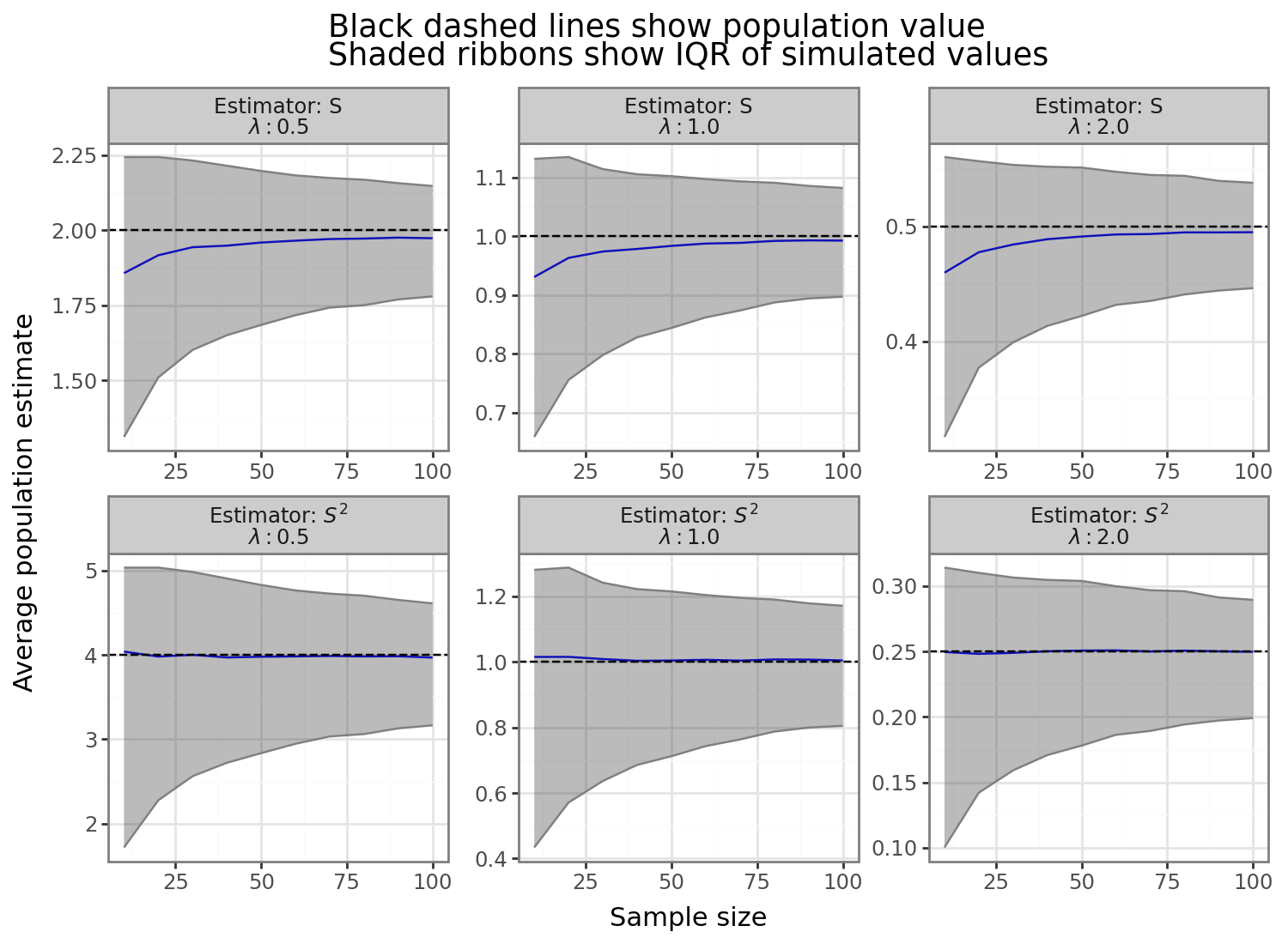
As the figure above shows, the sample variance (second panel row) is unbiased, despite being nonsymmetric, around the true population parameter for all three exponential distribution rates and for all sample sizes. In other words, \(S^2\) has a distribution that is non-normal but is mean zero relative to the population parameter. In contrast, the bias of the sample standard deviation is negative and inversely proportional to the sample size. Now that we’ve seen the problem of the negative bias inherent in the traditional, or “vanilla” sample SD estimator \(S\), the rest of the post will explore strategies for fixing it.
(2) Finite sample adjustment strategy
If \(E[S] \leq \sigma\) because of the concave square-root transform, then can some adjustment factor be applied to sample SD to correct for this? Specifically, we are interesting in finding some deterministic \(C_n\) such that:
\[\begin{align*} \sigma \approx C_n E[S] \tag{1}\label{eq:Cn_gaussian} \end{align*}\]Before further derivations, it should be intuitive that \(\underset{n\to \infty}{\lim} C_n = 1\), since the sample SD is consistent (but biased) and the exact form will vary for different parametric distributions.[2] The rest of this section proceeds as follows: first, I present the well-known solution for \(C_n\) when the data is Gaussian; second, I show how a series expansion can provide up to three-orders of analytic adjustments to account for the bias in \(S\).
(2.1) Normally distributed data
When \(X \sim N(\mu, \sigma^2)\), then an exact adjustment factor has been known since Holtzman (1950), and be calculated by simply working through the expectation of a power transformation of a chi-squared distribution (as the sample variance of Gaussian is chi-squared):
\[\begin{align*} S^2 &\sim \frac{\sigma^2}{n-1} \cdot \chi^2(n-1) \hspace{2mm} \text{ when $X$ is Gaussian} \\ E[Q^p] &= \int_0^\infty \frac{x^p x^{k/2-1} e^{-x/2}}{2^{k/2} \Gamma(k/2)} dx, \hspace{2mm} \text{ where } Q \sim \chi^2(k) \\ &= \frac{2^{p+k/2}}{2^{k/2} \Gamma(k/2)} \int_0^\infty z^{p+k/2-1} e^{-z} dz, \hspace{2mm} \text{ where } x = 2z \\ &= \frac{2^{m}}{2^{m-p} \Gamma(m-p)} \underbrace{\int_0^\infty z^{m-1} e^{-z} dx}_{\Gamma(m)}, \hspace{2mm} \text{ where } m = p + k/2 \\ &= 2^p \cdot \frac{\Gamma(k/2+p)}{\Gamma(k/2)} \\ E\Bigg[ \Bigg( \frac{(n-1)S^2}{\sigma^2} \Bigg)^{1/2} \Bigg] &= \frac{\sqrt{2} \cdot \Gamma(n/2)}{\Gamma([n-1]/2)} \\ E[ S ] &= \sigma \cdot \sqrt{\frac{2}{n-1}} \cdot \frac{\Gamma(n/2)}{\Gamma([n-1]/2)} \\ C_n &= \sqrt{\frac{n-1}{2}} \cdot \frac{\Gamma([n-1]/2)}{\Gamma(n/2)} \\ E[ S \cdot C_n ] &= \sigma \end{align*}\]Where \(\Gamma(\cdot)\) is the Gamma function. The code block below shows that this adjustment factor works as expected.
from scipy.special import gamma as GammaFunc
from scipy.special import gammaln as LogGammaFunc

# Adjustment factor
def C_n_gaussian(n: int, approx:bool = True) -> float:
    if approx:
        gamma_ratio = np.exp(LogGammaFunc((n-1)/2) - LogGammaFunc(n/2))
    else:
        gamma_ratio = GammaFunc((n-1)/2) / GammaFunc(n / 2)
    c_n = np.sqrt((n - 1)/2) * gamma_ratio
    return c_n

# Set up simulation parameters
nsim = 100000
sample_sizes = np.linspace(2, 50, num=25).astype(int)
mu = 1.3
sigma2 = 5
sigma = np.sqrt(sigma2)
dist_norm = norm(loc = mu, scale = sigma)
# Try sample STD
S_gauss_raw = np.vstack([dist_norm.rvs(size = (nsim, n), random_state=1).std(axis=1, ddof=1) for n in sample_sizes]).mean(axis=1)
S_gauss_adj = C_n_gaussian(sample_sizes) * S_gauss_raw
res_gauss = pd.DataFrame({'n':sample_sizes,'raw':S_gauss_raw, 'adj':S_gauss_adj}).\
    melt('n', var_name='msr', value_name='sd')

# Plot it
dat_adj_gauss = pd.DataFrame({'n':sample_sizes, 'adj':C_n_gaussian(sample_sizes)}).head(9)

pn.options.figure_size = (5.5, 3.5)
di_gauss_lbl ={'raw': 'Raw',
               'adj': 'Adjusted'}
gg_gauss = (pn.ggplot(res_gauss, pn.aes(x='n', y='sd', color='msr')) +
            pn.theme_bw() +
            pn.geom_line(size=2) +
            pn.geom_hline(yintercept=sigma, linetype='--') +
            pn.geom_text(pn.aes(label='(adj-1)*100', y=sigma*0.98), size=7, color='black', format_string='{:.0f}%', angle=90, data=dat_adj_gauss) +
            pn.scale_color_discrete(name='SD approach', labels = lambda x: [di_gauss_lbl[z] for z in x]) +
            pn.labs(y='Average sample SD', x='Sample size') +
            pn.ggtitle('Black dashed line show population SD\nText shows $100\cdot (C_n-1)$ for select sample sizes'))
gg_gauss
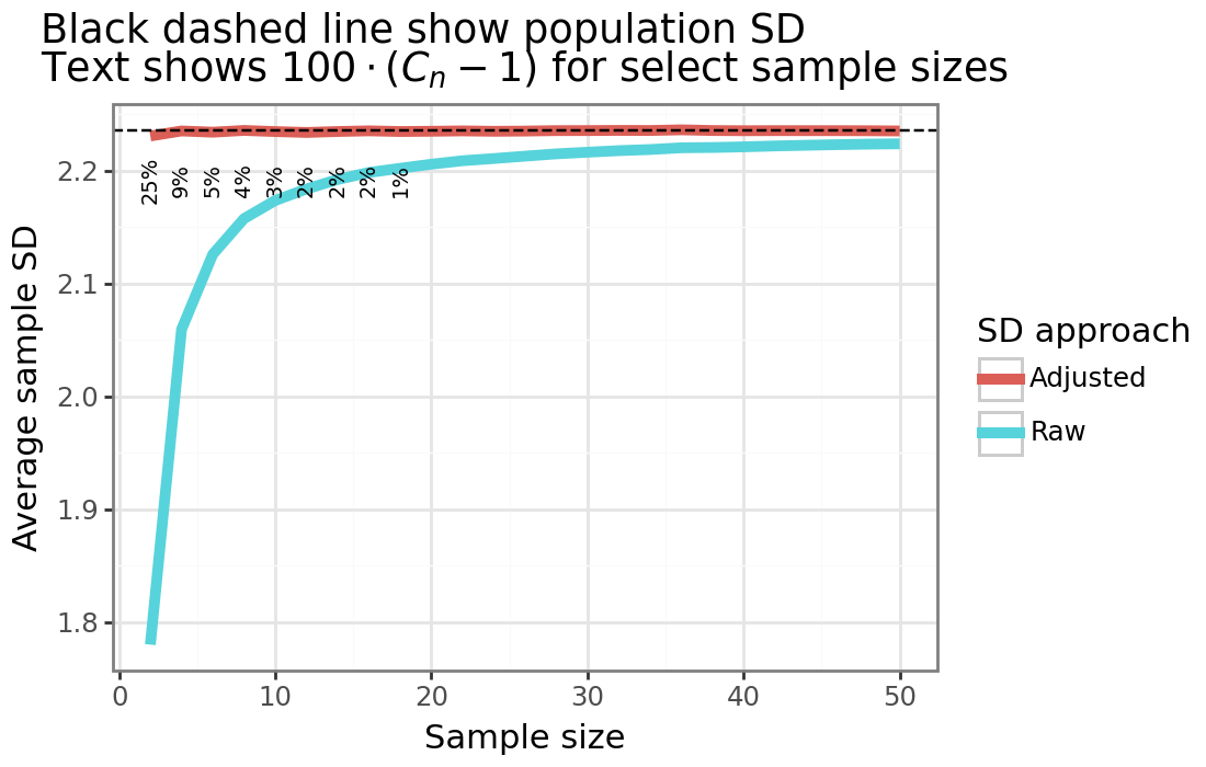
The figure above shows that the sample SD can be correctly adjusted for with \(C_n\) from \eqref{eq:Cn_gaussian} when the underlying data is normally distributed. When the sample size is small, this adjustment factor will be substantial (up to 25% when \(n=2\)). However, by around 20 samples, the adjustment factor will be 1% or less. Because \(C_n\) is only a function of \(n\), the same adjustment factor is true for all possible values of \((\mu, \sigma^2)\) which parameterize the normal distribution. When the data is Gaussian therefore, adjustments will be minimal, especially for large samples. As the rest of the post shows however, for non-Gaussian data, this is not always the case, and there can be a substantial bias even for large sample sizes.
(2.2) Non-normal data: approximations using a series expansion
For non-Gaussian data, the sample variance will not follow any well-defined distribution, and instead we’ll either need to appeal to asymptotic approximations or finite-sample adjustments. Because we already know that the sample SD is consistent, asymptotic approximation are not of interest, and instead this section will focus on Maclaurin Series expansions that can provide up to fourth-order approximations. As a starting step, \(S\) can be re-written as a function of \(\sigma\) (notice the RHS reduces to \(S\)):
\[S = \sigma [1 + (S^2 - \sigma^2)/\sigma^2]^{1/2}\]Next, consider the binomial series expansion:
\[(1 + x)^{0.5} = 1 + \frac{x}{2} - \frac{x^2}{8} + \frac{x^3}{16} - \frac{5 x^4}{128} + \dots\]Re-writing \(x = (S^2 - \sigma^2)/\sigma^2\) we see that:
\[S = \sigma \Bigg[1 + \frac{1}{2\sigma^2}(S^2 - \sigma^2) - \frac{1}{8\sigma^4}([S^2 - \sigma^2]^2) + \frac{1}{16\sigma^6}([S^2 - \sigma^2]^3) - \frac{5}{128\sigma^8}([S^2 - \sigma^2]^4) + \dots \Bigg]\]Now that we’ve re-written the sampling SD in terms of an infinite series and removed the square-root, we need to understand how fast the high-order terms tend towards zero as \(n\) increases. Remember, \(S^2\) is an unbiased estimator of \(\sigma^2\) so \(S^2-\sigma^2\) always averages to zero, and what we’re interested in understanding is how fast the variance decreases. For example, when \(X\) comes from a normal distribution, then:
\[\begin{align*} S^2 - \sigma^2 &= \sigma^2 \Bigg( \frac{\chi^2_{n-1}}{n-1} -1 \Bigg) \\ &\approx \sigma^2 \cdot N\Bigg(0, \frac{2}{n-1} \Bigg) \\ &\sim N\Bigg(0, \frac{2\sigma^4}{n-1} \Bigg), \end{align*}\]Where the second line uses the well-known fact that \(\chi^2_k \overset{d}{\to} N(k, 2k)\). What’s nice the sample variance follows a chi-square distribution asymptotically for any continuous RV, so we can use the above results for the sampling variance more generally:
\[\begin{align*} \frac{S^2 - \sigma^2}{\sigma^2} &\approx \sqrt{\frac{2}{\sigma(n-1)}} Z, \hspace{2mm} Z \sim N(0,1) \\ O\Bigg( \sqrt{\frac{2}{\sigma(n-1)}} Z \Bigg) &= O\Bigg( \frac{1}{\sqrt{n}} \Bigg) \\ O\Bigg( \frac{S^2 - \sigma^2}{\sigma^2}\Bigg) &= O(n^{-1/2}) \hspace{2mm} \longleftrightarrow \\ O\Bigg( \Bigg[ \frac{S^2 - \sigma^2}{\sigma^2} \Bigg]^k \Bigg) &= O(n^{-k/2}) \end{align*}\]We can see that the random variable \((S^2 - \sigma^2)/\sigma^2\) has a sampling error that is root-n consistent. And each time this term is raised to the power of \(k\), the sampling error decreases by a rate of \(k/2\). When \(n\) is large, then \(O(n^{-0.5})\) implies that that the sample size needs increase by 4x, for the estimator’s standard error to fall by 1/2. Whereas for \(O(n^{-1})\) and \(O(n^{-1.5})\) when the sample size doubles and increases by 59%, respectively, the standard error will half. More generally, the formula to halve the SE will be: \(n’ = 2^{k / 2} n\), or alternatively, for a doubling of the sample size, the SE will decrease by: \(2^{-k/2}\).
Let’s check that this is indeed true for the exponential distribution: namely, when \(n\) is large, if \(n’ = 2n\), then does the standard error of \((S^2 - \sigma^2)/\sigma^2\) decrease by around \(2^{-k/2}\)? In the simulation below we’ll use the same three rate parameters for the exponential distribution described above, and compare \(\text{SE}(S^2_{n’})/\text{SE}(S_n^2)\) when \(n=1000\) vs \(n’=2000\) over 2500 simulations and see if it equal to \(2^{-k/2}\) for \(k \in {1, 2, 3, 4}\).
# Set up terms
nsim = 2500
n = 1000
nprime = int(2 * n)
# Draw exponential data and calculate sample variance
S2_n = dist_expon.rvs(size = (n, nsim, n_rates), random_state=1).var(ddof=1, axis=0)
S2_nprime = dist_expon.rvs(size = (nprime, nsim, n_rates), random_state=2).var(ddof=1, axis=0)
# Normalize to oracle variance
norm_var_n = (S2_n - oracle_variance) / oracle_variance
norm_var_nprime = (S2_nprime - oracle_variance) / oracle_variance
# Calculate the theoretical decrease
rate_theory = pd.DataFrame({'k':[1, 2, 3, 4]}).assign(theory=lambda x: 2**(-x['k']/2))

# Calculate the relative variance
res_order = np.vstack([np.std(norm_var_nprime**k, axis=0, ddof=1) / np.std(norm_var_n**k, axis=0, ddof=1) for k in rate_theory['k']])
res_order = pd.DataFrame(res_order.T, columns=rate_theory['k'], index=rates).rename_axis('rate')
res_order = res_order.melt(ignore_index=False, value_name='emp').reset_index()
res_order = res_order.merge(rate_theory)

pn.options.figure_size = (5.5, 3.5)
gg_se_theory = (pn.ggplot(res_order, pn.aes(x='theory', y='emp', color='k.astype(str)', shape='rate.astype(str)'))+
          pn.theme_bw() + pn.geom_point() +
          pn.labs(y='Empirical SE reduction', x='Theory') +
          pn.ggtitle('Dashed line shows y==x\nTheory shows $2^{-k/2}$') +
          pn.scale_color_discrete(name='k') +
          pn.scale_shape_discrete(name='Rate ($\\lambda$)') +
          pn.geom_abline(slope=1, intercept=0,linetype='--'))
gg_se_theory
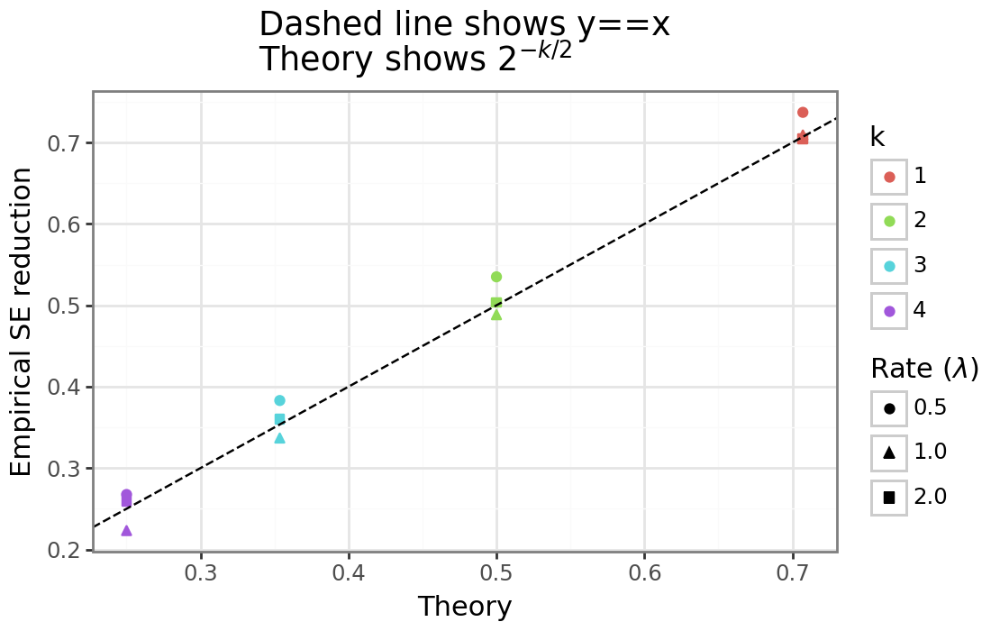
The figure above shows that we achieve the variance reduction close to what was expected. As \(n\) and the number of simulations gets larger, the results will become increasingly exact.[3]
If we approximate \(S\) up to \(k=4\) then the remainder term will disappear at a rate of \(O(n^{2.5})\); i.e. very quickly.
\[S = \sigma \Bigg[1 + \frac{1}{2}\frac{S^2 - \sigma^2}{\sigma^2} - \frac{1}{8}\Big(\frac{S^2 - \sigma^2}{\sigma^2}\Big)^2 + \frac{1}{16}\Big(\frac{S^2 - \sigma^2}{\sigma^2}\Big)^3 - \frac{5}{128}\Big(\frac{S^2 - \sigma^2}{\sigma^2}\Big)^4 \Bigg] + O(n^{-2.5})\]Next, we can calculate the expected value of this fourth-order approximation (note that \(E[S^2 - \sigma^2] = 0\)):
\[E[S] \approx \sigma \Bigg[1 - \frac{1}{8}\Big(\frac{E[S^2 - \sigma^2]^2}{\sigma^4}\Big) + \frac{1}{16}\Big(\frac{E[S^2 - \sigma^2]^3}{\sigma^6}\Big) - \frac{5}{128}\Big(\frac{E[S^2 - \sigma^2]^4}{\sigma^8}\Big) \Bigg]\]While it’s not exactly clear what \(E[S^2 - \sigma^2]^k\) would be in general, luckily, existing work by Angelova (2012) has already done this up to \(k=4\) (see equation 19), which is shown below and spaced for readability for convenience.
\[\begin{align*} \mu_k &= E[X - E(X)]^k \\ \mu_{2,S^2} &= E[S^2 - \sigma^2]^k \\ \mu_{2,S^2} &= \frac{(\mu_4 - \mu_2^2)}{n} + \frac{2\mu_2^2}{n(n-1)} \\ \mu_{3,S^2} &= \frac{(\mu_6 - 3\mu_4\mu_2 - 6\mu_3^2 + 2\mu_2^3)}{n^2} + \frac{4(3\mu_4\mu_2 - 5\mu_2^3)}{n^2(n-1)} - \frac{4(\mu_3^2 - 2\mu_2^3)}{n^2(n-1)^2} \\ \mu_{4,S^2} &= \frac{3(\mu_4 - \mu_2^2)^2}{n^2} \\ &\quad + \frac{(\mu_8 - 4\mu_6\mu_2 - 24\mu_5\mu_3 - 3\mu_4^2 + 24\mu_4\mu_2^2 + 96\mu_3^2\mu_2 - 18\mu_2^4)}{n^3} \\ &\quad + \frac{12(2\mu_6\mu_2 + 2\mu_4^2 - 17\mu_4\mu_2^2 - 12\mu_3^2\mu_2 + 18\mu_2^4)}{n^3(n-1)} \\ &\quad - \frac{4(8\mu_5\mu_3 - 36\mu_4\mu_2^2 - 56\mu_3^2\mu_2 + 69\mu_2^4)}{n^3(n-1)^2} \\ &\quad + \frac{8(\mu_4^2 - 6\mu_4\mu_2^2 - 12\mu_3^2\mu_2 + 15\mu_2^4)}{n^3(n-1)^3} \end{align*}\]We can now formally define the \(k^{th}\) order adjustment for the sample SD:
\[\begin{align*} C_n(k) &= \begin{cases} 1 & \text{ if } k = 1 \\ \Bigg[1 + \sum_{j=2}^k \binom{\frac{1}{2}}{j} \frac{\mu_{j, S^2}}{\sigma^{(2j)}} \Bigg]^{-1} \hspace{2mm} & \text{ for } k \in \{2, 3, 4\} \tag{2}\label{eq:Cn_l} \end{cases} \end{align*}\]Note that Giles (2021) defines \eqref{eq:Cn_l} for \(k=2\), which can be written as a function of the empirical kurtosis. To make the approach more modular, I have left the terms as they are (i.e. not re-factored as central moments like kurtosis). This means that were an oracle calculating \(C_n\) for up to \(k=4\), it would need to know the central moments of \(X\) up to eighth power. In practice, estimates of each will need to be provided from the data. When the parametric form of \(X\) is known, then the central moments will usually be a function of that distribution’s population parameter(s) and can be substituted in for a simple MLE estimate. When \(X\) comes from an unknown distribution, then the empirical moments will need to be provided. In either case, there will be a bias/variance trade-off, and using \(C_n(1)=S\) may be better than \(C_n(k)\) for \(k \geq 2\).
(2.3) Oracle adjustment for the exponential distribution
Before having to actually estimate \(C_n(k)\) with data, let us first examine how much bias is removed when it calculated analytically in the case of an exponential distribution. This distribution’s central moments can be analytically written as a function of its rate parameter: \(\mu_k(\lambda) = \frac{k!}{\lambda^k} \sum_{j=0}^k \frac{(-1)^j}{j!}\). The first code block below provides a python implementation for both the central moment generator of an exponential distribution as well as a generic function to calculate \(\mu_{k,S^2}\) when a moment_func is provided values for \(k \in {1, 2, 3, 4}\).
from math import factorial
from scipy.special import binom
from typing import Callable, Tuple, List

class CentralExpMoments:
    def __init__(self, lambd: float):
        """
        Calculates the central moments of an exponential distribution for same rate parameter (lambd): X ~ Exp(lambd)

        \mu_k(\lambda) = E[(X - E(X))^k] = \frac{k!}{\lambda^k} \sum_{j=0}^k \frac{(-1)^j}{j!}
        """
        self.lambd = lambd

    def __call__(self, k: int) -> float:
        """Return the k'th central moment"""
        factorial_k = factorial(k)
        sum_term = sum(((-1)**j) / factorial(j) for j in range(k + 1))
        moment = (factorial_k / (self.lambd**k)) * sum_term
        return moment


def mu_k_S2(k:int | List | Tuple, n: int, moment_func: Callable) -> np.ndarray:
    """
    Calculate \mu_{k, S^2} = E[(S^2 - \sigma^2)]^k for k={1,2,3,4}

    Args
    ====
    k: int
        A list of orders to calculate (or a single term if int)
    n: int
        The sample size
    moment_func:
        A function to calculate the (central) moment for the assumed distribution of X where moment_func(k) = E[(E-E(X))^k]
    """
    # Input checks
    valid_k = [1, 2, 3, 4]
    if isinstance(k, int):
        k = [k]
    assert all([j in valid_k for j in k]), f'k must be one {valid_k}'
    k_max = max(k)

    # Calculate necessary moments
    if k_max >= 2:
        mu2 = moment_func(2)
        mu3 = moment_func(3)
        mu4 = moment_func(4)
    if k_max >= 3:
        mu5 = moment_func(5)
        mu6 = moment_func(6)
    if k_max == 4:
        mu8 = moment_func(8)

    # Calculate the adjustment terms
    val = []
    if 1 in k:
        mu_1_S2 = 0
        val.append(mu_1_S2)
    if 2 in k:
        mu_2_S2 = (mu4 - mu2**2) / n + 2 * mu2**2 / (n * (n - 1))
        val.append(mu_2_S2)
    if 3 in k:
        mu_3_S2 = (mu6 - 3 * mu4 * mu2 - 6 * mu3**2 + 2 * mu2**3) / n**2 + \
             4 * (3 * mu4 * mu2 - 5 * mu2**3) / (n**2 * (n - 1)) - \
             4 * (mu3**2 - 2 * mu2**3) / (n**2 * (n - 1)**2)
        val.append(mu_3_S2)
    if 4 in k:
        mu_4_S2 = 3 * (mu4 - mu2**2)**2 / n**2 + \
                (mu8 - 4 * mu6 * mu2 - 24 * mu5 * mu3 - 3 * mu4**2 + 24 * mu4 * mu2**2 + 96 * mu3**2 * mu2 - 18 * mu2**4) / n**3 + \
                12 * (2 * mu6 * mu2 + 2 * mu4**2 - 17 * mu4 * mu2**2 - 12 * mu3**2 * mu2 + 18 * mu2**4) / (n**3 * (n - 1)) - \
                4 * (8 * mu5 * mu3 - 36 * mu4 * mu2**2 - 56 * mu3**2 * mu2 + 69 * mu2**4) / (n**3 * (n - 1)**2) + \
                8 * (mu4**2 - 6 * mu4 * mu2**2 - 12 * mu3**2 * mu2 + 15 * mu2**4) / (n**3 * (n - 1)**3)
        val.append(mu_4_S2)

    val = np.array(val)
    return val
To make sure that mu_k_S2 works as expected, we can compare the average value of the difference between the sample variance and the population variance to the powers of 1, 2, 3, and 4 for 1-million simulations and compare to this values expected from \(\mu_{k,S^2}\) when the data is drawn from \(X \sim \text{Exp}(2)\) and the central moments known with oracle precision.
from scipy.stats import ttest_1samp
# Set up parameters
seed = 1234
lambd = 2
sample_size = 2
nsim = 1000000
Xdist = expon(scale = 1 / lambd)
k_orders = [1, 2, 3, 4]
# Calculate population/oracle values
sigma2 = Xdist.var()
central_Exp_moments = CentralExpMoments(lambd = lambd)
theory_mu_S2 = mu_k_S2(k = k_orders, n = sample_size, moment_func=central_Exp_moments)

# Draw data and calculate sample variance
S2 = Xdist.rvs(size = (nsim, sample_size), random_state=seed).var(axis=1, ddof=1)
hat_mu_S2 = np.array([np.mean((S2 - sigma2)**k) for k in k_orders])
pval_mu_1_S2 = np.array([ttest_1samp(a = (S2 - sigma2)**k, popmean=theory_mu_S2[i]).pvalue for i,k in enumerate(k_orders)])
# Show that results are within theory
pd.DataFrame({'k':k_orders,
              'Theory':theory_mu_S2,
              'Empirical':hat_mu_S2,
              'P-value':pval_mu_1_S2}).round(4)
| k | Theory | Empirical | P-value | |
|---|---|---|---|---|
| 0 | 1 | 0.0000 | -0.0005 | 0.3988 |
| 1 | 2 | 0.3125 | 0.3076 | 0.0770 |
| 2 | 3 | 1.1562 | 1.0984 | 0.0793 |
| 3 | 4 | 8.5664 | 7.6422 | 0.1143 |
As expected, the empirical averages are statistically indistinguishable from the theoretical mean showing that Angelova (2012) derivations hold. The next code block provides the C_n_adj function which takes in a value of k and a moment_func and returns the adjustment factor.
from mizani.formatters import percent_format

def C_n_adj(k:int, n: int, moment_func: Callable) -> float | Tuple:
    """
    Calculate the adjustment factor for: C_n(k) &= \Bigg[1 + \sum_{j=2}^k \binom{\frac{1}{2}}{j} \frac{\mu_{k, S^2}}{\sigma^{(2k)}} \Bigg]^{-1}

    Args
    ====
    k: int
        A list of orders to calculate (or a single term if int)
    n: int
        The sample size
    moment_func:
        A function to calculate the (central) moment for the assumed distribution of X where moment_func(k) = E[(E-E(X))^k]
    """
    # Input checks
    assert k in [1, 2, 3, 4], 'k needs to be {1, 2, 3, 4}'
    assert isinstance(n, int), 'n needs to be an int'
    if k == 1:
        return 1  # no adjustmemt needed
    k_seq = list(range(2, k + 1))
    # Calculate the E[S^2 - sigma^2]^k and sigma^2
    mu_k_seq = mu_k_S2(k=k_seq, n=n, moment_func=moment_func)
    sigma2 = moment_func(2)
    # Calculate the adjustment term
    coef_binom = np.array([binom(0.5, j) for j in k_seq])
    sigma2_seq = np.array([sigma2 ** j for j in k_seq])
    C_n = 1 / (1 + np.sum(coef_binom * mu_k_seq / sigma2_seq))
    return C_n

# Run the simulations
nsim = 100000
k_seq = [1, 2, 3, 4]
sample_sizes = np.arange(5, 100+1, 5)
# Calculate adjustment factors
adjust_factors = np.vstack([np.array([C_n_adj(k=k, n=int(n), moment_func=central_Exp_moments) for n in sample_sizes]) for k in k_seq]).T
# Calculate the average sample SD
S_hat_bar = np.vstack([dist_expon.rvs(size = (nsim, n, n_rates), random_state=seed).std(axis=1, ddof=1).mean(axis=0) for n in sample_sizes])
S_hat_bar_adj = np.expand_dims(S_hat_bar, 2) * np.expand_dims(adjust_factors,1)
# Calculate the percentage error to population param
pct_deviation = S_hat_bar_adj / np.atleast_3d(np.sqrt(dist_expon.var())) - 1
res_pct_deviation = pd.concat(objs=[pd.DataFrame(pct_deviation[:,:,j],index=sample_sizes,columns=rates).assign(k=k) for j,k in enumerate(k_seq)])
res_pct_deviation.rename_axis('sample_size', inplace=True)
res_pct_deviation.set_index('k',append=True, inplace=True)
res_pct_deviation = res_pct_deviation.melt(ignore_index=False, var_name='lambd', value_name='pct')
res_pct_deviation.reset_index(inplace=True)

di_k = {str(k):f'$C_n({k})$' for k in k_seq}
pn.options.figure_size = (10, 3.5)
di_rates = {str(r):f'$\\lambda: {r}$' for r in rates}
gg_pct_dev = (pn.ggplot(res_pct_deviation, pn.aes(x='sample_size', y='pct.abs()', color='k.astype(str)')) +
              pn.theme_bw() + pn.geom_line() +
              pn.scale_y_log10(labels=percent_format()) +
              pn.scale_x_continuous(limits=[0, max(sample_sizes)]) +
              pn.facet_wrap('~lambd', nrow=1, labeller=pn.labeller(cols=lambda x: di_rates[x])) +
              pn.geom_hline(yintercept=res_pct_deviation.pct.abs().min()*0.5, linetype='--') +
              pn.scale_color_discrete(name='Order',labels = lambda x: [di_k[z] for z in x]) +
              pn.labs(y='Absolute bias (%)', x='Sample size') +
              pn.ggtitle('Effect of oracle $C_n(k)$ on SD bias'))
gg_pct_dev
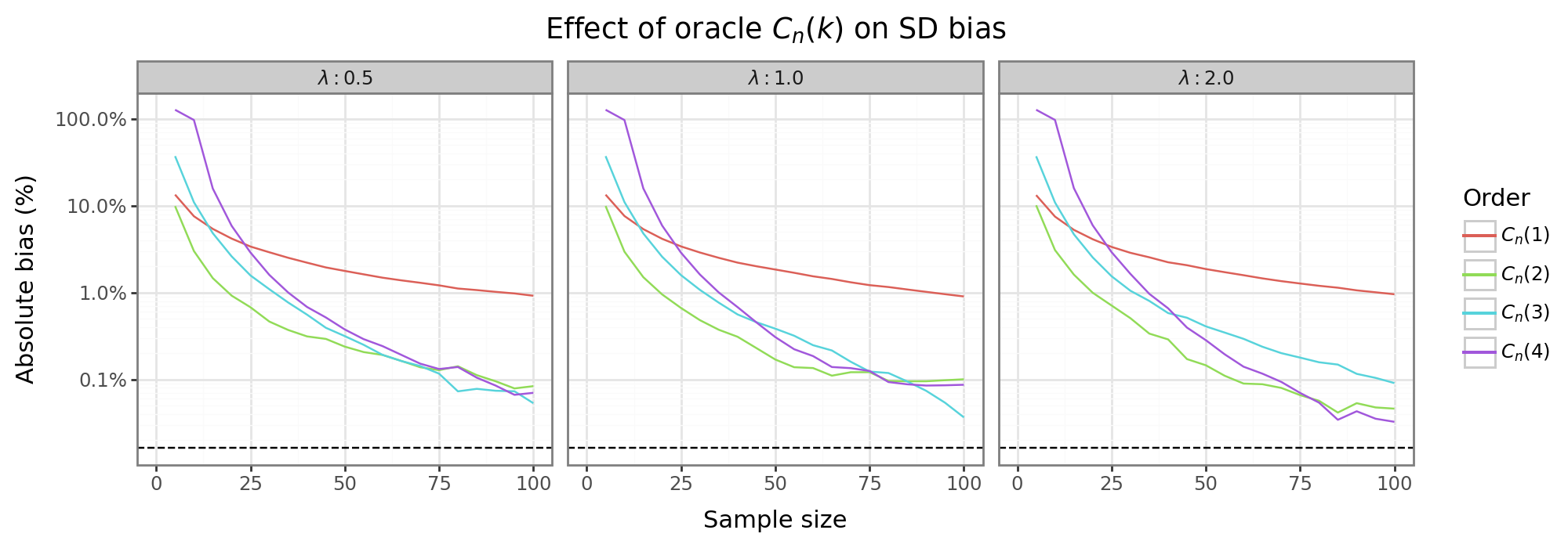
The figure above shows the absolute bias (on the log scale) of the sample SD after the oracle adjustment for the SDs of the three different exponential distributions; i.e. \(|\frac{\hat{\sigma}}{\sigma} - 1|\). For small sample sizes, the second and third order adjustments, \(C_n({3,4})\), are more biased than the vanilla sample SD: \(C_n(1)\). This is not that surprising since the binomial series expansion only converges when \(x < 1\), so \(|[S^2 - \sigma^2]^k/\sigma^{2k}|<1\). For small \(n\) the expansion may therefore not be stable. In contrast, the first order adjustment (\(C_n(2)\)) always dominates the vanilla SD. Are higher order adjustments ever preferable over the first order adjustment? In this example, somewhere around \(n=75\), using higher order oracle adjustment can decrease the bias, but only marginally. The fact that in these terms will need to estimated in applied settings means that in practice, the only feasible SD estimators will be vanilla or first-order adjustment.
(2.4) Bias-variance trade-off
Section (2.3) showed that even with oracle precision, second- and third-order adjustments are unlikely to be helpful with combating the bias of the sample SD. Therefore, this section will focus on comparing the vanilla SD with the first-order adjustment, as the latter dominates in the oracle situation. However, once we actually need to estimate the terms that go into this adjustment, it’s not clear a priori whether it will be a better estimator. The reasons for this are two-fold. First, the adjustment term requires estimating a higher-order moment of the distribution. Just as estimating the SD with its sample counterpart leads to a biased estimator, the estimators for the fourth moment or variance squared will also be biased. Second, even if the terms could be estimated without any bias, the variance of the estimator will necessarily be larger. We can therefore think about the quality of the estimator in terms of the expected value of a loss function like the mean squared error or mean absolute error. This expected value, the risk of the estimator, will therefore have a bias-variance trade-off for which the rest of this section will explore.
Focusing on the first-order expansion, we can simplify the terms seem in equation \eqref{eq:Cn_l}:
\[\begin{align*} \sigma &\approx E[S] \cdot \underbrace{\Bigg[1 - \frac{1}{8n}\Bigg(\kappa - 1 + \frac{2}{(n-1)} \Bigg) \Bigg]}_{C_n^{-1}(2)} \tag{3}\label{eq:Cn_kappa} \end{align*}\]So that the adjustment factor is a function of the sample size, \(n\), and the kurtosis, \(\kappa = E[(X - \mu)^4/\sigma^4]\). This population parameter can estimated non-parametrically. If one “knows” the parametric form of the data, then the kurtosis may be a function of the population parameters.
(2.4.1) Kurtosis estimator
This subsection will first analyze the bias and variance of estimating the kurtosis necessary for calculating the adjustment in equation \eqref{eq:Cn_kappa}, when the data is drawn from a binomial distribution. The kurtosis will be estimated with both parametric and non-parametric approaches. Denote a draw from the binomial distribution as \(X \sim \text{Bin}(p,m)\), where \(p\) is the probability of success and \(m\) is the number of draws. It is easy to show that the kurtosis is a function of the population parameters: \(\text{Kurt}(X)=\kappa = 3 - 6/m + [mp(1-p)]^{-1}\). Since \(m\) is assumed to be known, after \(p\) is estimated, a “plug-and-play” estimate is derived. For the non-parametric case, we can use either the adjusted or unadjusted approaches for estimating kurtosis:[4]
\[\begin{align*} \kappa^{\text{para}} &= 3 - 6/m + [m\cdot\hat{p}\cdot(1-\hat{p}) ]^{-1} \\ \hat{p} &= n^{-1} \sum_{i=1}^n (X_i / m) \\ \kappa^{\text{unj}} &= \frac{n^{-1}\sum_{i=1}^n (X_i - \bar{X})^4}{\Big[n^{-1}\sum_{i=1}^n (X_i - \bar{X})^2 \Big]^2} \\ \kappa^{\text{adj}} &= \frac{(n^2-1)\kappa^{\text{unj}} - 9n + 15}{(n-2)(n-3)} \end{align*}\]The code below rune 100K simulations for estimating the (known) kurtosis for a binomial distribution with \(p \in {0.1, 0.3, 0.5 }\) and \(m=20\) for sample sizes between \({ 5, 10, \dots, 50 }\). The average squared error (MSE), absolute error (MAE), bias, and variance is shown for the there different estimators shown above.
# Load extra functions
from scipy.stats import binom, kurtosis
from mizani.palettes import hue_pal

# Set up binomial distribution
seed = 2
nsim = 100000
sample_sizes = np.arange(5, 50 + 1, 5)
m = 20
p_seq = [0.1, 0.3, 0.5]
n_p = len(p_seq)
dist_binom = binom(n=m, p=p_seq)
# scipy defines kurtosis as "excess" relative to the Gaussian, so add back 3
kappa0 = dist_binom.stats('k') + 3
dat_kappa0 = pd.DataFrame({'p':p_seq, 'kappa':kappa0})
# Loop over the different sample sizes
holder_binom = []
for sample_size in sample_sizes:
    # Draw data
    X = dist_binom.rvs(size=[sample_size, nsim, n_p], random_state=seed)
    Xbar = X.mean(axis=0)
    mu4 = np.mean((X - Xbar)**4, axis=0)
    mu22 = np.mean((X - Xbar)**2, axis=0)**2
    # Calculate different kappa variants
    p = Xbar / m
    p[p == 0] = 1 / m
    kappa_para =  3 - 6/m + 1/(m*p*(1-p))
    kappa_np_unj = kurtosis(a=X, fisher=False, bias=True, axis=0)
    kappa_np_adj = kurtosis(a=X, fisher=False, bias=False, axis=0)
    # Check that it aligns with expectation
    np.testing.assert_almost_equal(kappa_np_unj, mu4 / mu22)
    np.testing.assert_almost_equal(kappa_np_adj, ( (sample_size**2-1)*mu4/mu22 - 9*sample_size + 15 ) / ((sample_size-2)*(sample_size-3)) )
    # Calculate the bias/variance/MSE/MAE
    di_kappa = {'para':kappa_para, 'np_unj':kappa_np_unj, 'np_adj':kappa_np_adj}
    res_kappa = pd.concat(objs=[pd.DataFrame(pd.DataFrame(v, columns=p_seq).assign(method=k)) for k,v in di_kappa.items()])
    res_kappa = res_kappa.melt('method', var_name='p').merge(dat_kappa0)
    res_kappa = res_kappa.groupby(['method','p']).apply(lambda x: pd.Series({
        'bias': np.mean(x['kappa'] - x['value']),
        'variance': np.var(x['kappa'] - x['value']),
        'MSE': np.mean((x['kappa'] - x['value'])**2),
        'MAE': np.mean(np.abs(x['kappa'] - x['value']))})
    )
    res_kappa = res_kappa.melt(ignore_index=False, var_name='msr').reset_index()
    res_kappa.insert(0, 'n', sample_size)
    del di_kappa, kappa_para, kappa_np_unj, kappa_np_adj
    holder_binom.append(res_kappa)

# Merge all results
res_kappa = pd.concat(holder_binom)

# Plot results
di_method = {'np_adj':'$\\kappa^{\\text{adj}}$',
             'np_unj':'$\\kappa^{\\text{unj}}$',
             'para': '$\\kappa^{\\text{para}}$'}
di_msr = {'bias':'Bias',
          'variance': 'Variance',
          'MSE':'MSE', 'MAE':'MAE'}
di_p = {str(p):f'p={p:.2f}' for p in p_seq}

colorz = hue_pal()(3)
pn.options.figure_size = (10, 6.5)
gg_kappa = (pn.ggplot(res_kappa, pn.aes(x='n', y='value', color='method')) +
            pn.theme_bw() + pn.geom_line() +
            pn.labs(x = 'Sample size', y='Average measure over simulations') +
            pn.scale_x_continuous(limits=[0, sample_sizes[-1]]) +
            pn.ggtitle(f'Kurtosis estimator performance for Bin(m,p)\n$m={m}$, simulations={nsim:,}') +
            pn.scale_color_manual(name='Method', labels=lambda x: [di_method[z] for z in x], values=colorz) +
            pn.facet_grid('p~msr', labeller=pn.labeller(rows=lambda x: di_p[x], cols = lambda x: di_msr[x]),scales='free_y')
            )
gg_kappa
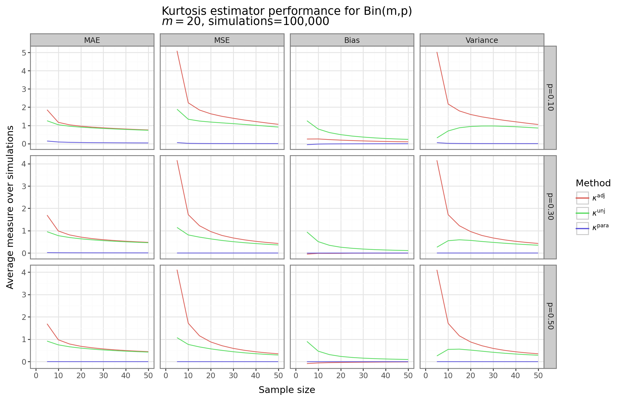
The figure above shows four different measures of the kurtosis estimator performance for three different parameter values of the binomial distribution for the parametric and non-parametric approaches as a function of the sample size. As would be expected, all estimators decrease their MSE and MAE as the sample size increases. However, the parametric “plug-and-play” approach dominates. This shows that when the parametric form of the data is known, and an analytical expression for the kurtosis can be written in terms of its parameters estimable by MLE, then the parametric kurtosis estimator is likely the sensible choice.[5]
For the non-parametric approaches, the unadjusted approach, interestingly, does better in terms of MAE/MSE. The reason for this can be seen in the “Bias” and “Variance” columns. While the unadjusted approach has much higher bias (indeed both the parametric and adjusted methods have close to zero bias for these three binomial distributions), its variance is substantially lower that the adjusted approach. For example, when \(n=5\), then the adjustment factor is four, and the variance is concomitantly sixteen-fold higher for the adjusted method.
While this section has shown the relative merits of the different kurtosis estimators, we need to check how they fare when actually estimating the SD of a distribution, which is the purpose of this post after all.
(2.4.2) Binomial SD
We will continue our binomial distribution example and this time focus on the same four measures of estimator performance (MSE, MAE, variance, bias) but for the distribution’s SD, rather than its kurtosis. While a noisier kurtosis estimator will increase the MSE/MAE, ceteris paribus, the final MSE/MAE for the SD will depend on the relative magnitude of the variance, and the relative change in the bias of the SD.
The code below runs create a new function sd_adj which will use the first-order approximation when kappa is provided from \eqreq{eq:Cn_kappa}. The simulation parameters are the same as the binomial distribution described above.
def sd_adj(x: np.ndarray, kappa: np.ndarray | None = None, ddof:int = 1, axis: int | None = None) -> np.ndarray:
    """
    Adjust the vanilla SD estimator
    """
    std = np.std(x, axis=axis, ddof = ddof)
    nrow = x.shape[0]
    if kappa is not None:
        adj = 1 / ( 1 - (kappa - 1 + 2/(nrow-1)) / (8*nrow) )
        std = std * adj
    return std

sim_perf = lambda x: pd.Series({
        'mu': np.mean(x['value']),
        'bias': np.mean(x['value'] - x['sd']),
        'variance': np.var(x['sd'] - x['value']),
        'MSE': np.mean((x['sd'] - x['value'])**2),
        'MAE': np.mean(np.abs(x['sd'] - x['value']))})

# Calculate the population SD
dat_sd_binom = pd.DataFrame({'p':p_seq, 'sd':np.sqrt(dist_binom.stats('v'))})

# Loop over each sample size
holder_binom = []
for sample_size in sample_sizes:
    # Draw data
    X = dist_binom.rvs(size=[sample_size, nsim, n_p], random_state=seed)
    # Calculate different kappa variants
    p = X.mean(axis = 0) / m
    p[p == 0] = 1 / (m + 1)
    kappa_para =  3 - 6/m + 1/(m*p*(1-p))
    kappa_np_unj = kurtosis(a=X, fisher=False, bias=True, axis=0)
    kappa_np_adj = kurtosis(a=X, fisher=False, bias=False, axis=0)
    # Estimate the SD
    sigma_vanilla = sd_adj(x=X, axis=0)
    sigma_para = sd_adj(x=X, axis=0, kappa=kappa_para)
    sigma_unj = sd_adj(x=X, axis=0, kappa=kappa_np_unj)
    sigma_adj = sd_adj(x=X, axis=0, kappa=kappa_np_adj)
    # Calculate the bias/variance/MSE/MAE
    di_sigma = {'vanilla':sigma_vanilla, 'para':sigma_para,
                'np_unj':sigma_unj, 'np_adj':sigma_adj}
    res_sigma = pd.concat(objs=[pd.DataFrame(pd.DataFrame(v, columns=p_seq).assign(method=k)) for k,v in di_sigma.items()])
    res_sigma = res_sigma.melt('method', var_name='p').merge(dat_sd_binom)
    res_sigma = res_sigma.groupby(['method','p']).apply(sim_perf)
    res_sigma = res_sigma.melt(ignore_index=False, var_name='msr').reset_index()
    res_sigma.insert(0, 'n', sample_size)
    del di_sigma, sigma_vanilla, sigma_para, sigma_unj, sigma_adj
    holder_binom.append(res_sigma)
# Merge results
res_sd_binom = pd.concat(holder_binom)

# Plot the performance
di_method = {**{'vanilla':'Vanilla'}, **di_method}

# Subset the dat
dat_plot = res_sd_binom.query('msr!= "mu"').copy()

colorz = hue_pal()(3) + ['black']
pn.options.figure_size = (10, 6.5)
gg_perf_binom = (pn.ggplot(dat_plot, pn.aes(x='n', y='value', color='method')) +
            pn.theme_bw() + pn.geom_line() +
            pn.labs(x = 'Sample size', y='Average measure over simulations') +
            pn.scale_x_continuous(limits=[0, sample_sizes[-1]]) +
            pn.ggtitle(f'SD estimator performance for Bin(m,p)\n$m={m}$, simulations={nsim:,}') +
            pn.scale_color_manual(name='Method', labels=lambda x: [di_method[z] for z in x], values=colorz) +
            pn.facet_wrap('~p+msr', labeller=pn.labeller(cols = lambda x: {**di_p, **di_msr}[x]), scales='free_y')
            )
gg_perf_binom
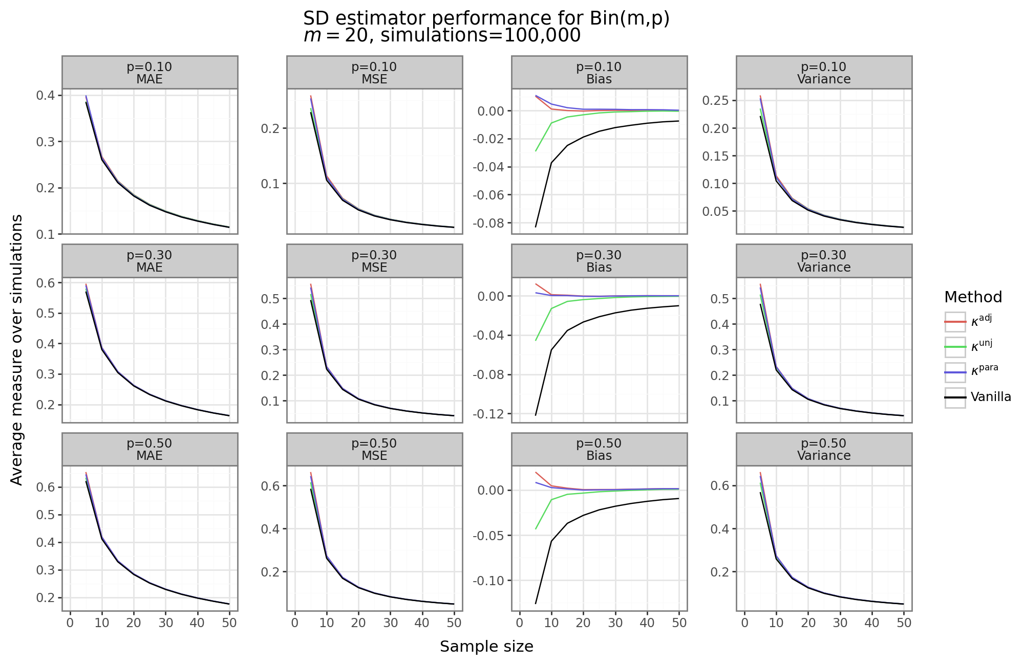
The figure above shows that the MAE/MSE for almost all of our kurtosis estimators is largely the same. While the bias for all of the adjustment methods is better, the magnitude of this bias is dwarfed by the variance of SD estimator. The vanilla estimator (i.e. square-root of the sample variance), has highest bias, the lowest variance, and the lowest MAE/MSE. The parametric method dominates the adjusted non-parametric approach in that it has slightly less bias but lower variance. However, the non-adjusted non-parametric approach, like the vanilla estimator, has higher bias than either the parametric or adjustment approach, but lower variance and a lower MSE/MAE. Hence, for use cases where having a biased estimator is problematic, and we are willing to pay for it with a bit of variance, any one of our adjustment methods could be worth it.[6]
# Plot the actual vs oracle
dat_plot = res_sd_binom.query('msr == "mu"').merge(dat_sd_binom)

pn.options.figure_size = (11, 3.5)
gg_sd_binom = (pn.ggplot(dat_plot, pn.aes(x='n', y='value', color='method')) +
            pn.theme_bw() + pn.geom_line() +
            pn.facet_wrap(facets='~p', scales='free', labeller=pn.labeller(cols = lambda x: di_p[x])) +
            pn.scale_color_manual(name='Method', labels=lambda x: [di_method[z] for z in x], values=colorz) +
            pn.geom_hline(pn.aes(yintercept='sd'), data=dat_sd_binom, linetype='--') +
            pn.labs(y='Average SD estimate over simulations', x='Sample size') +
            pn.scale_x_continuous(limits=[0, dat_plot['n'].max()]) +
            pn.ggtitle('Black dashed lines show population SD'))
gg_sd_binom
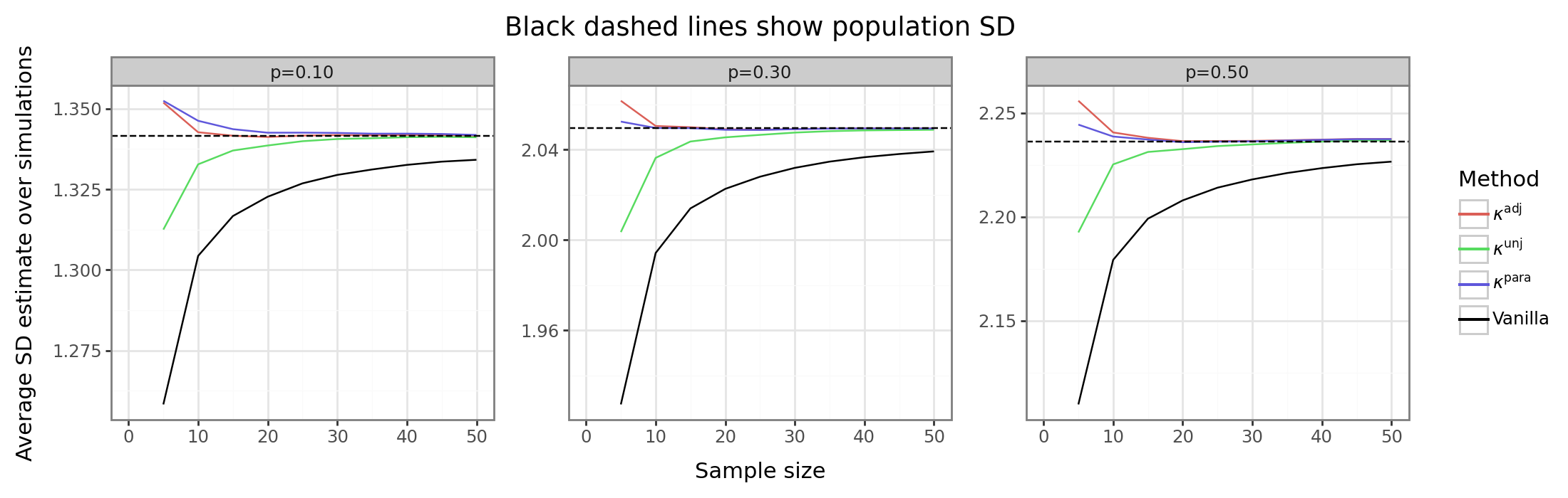
This next figure shows the average SD estimate over all simulation runs compared to the population parameter. Interestingly, we see that the while the use of the first-order adjustment reduces the bias, only the parametric or adjusted methods yield a conservative estimator, while the unadjusted method yields an optimistic estimator, albeit less biased than the unadjusted method. This distinction is important because there may be contexts when we prefer the bias to be one direction over another. For example, if the SD is used as a way to generate a type of z-score, then an optimistic estimator may have inflated type-I errors, whereas a conservative estimator will have deflated type-I errors and reduced power.
(3) Non-parametric adjustment strategies
The examined approaches so far have relied on finding a functional form of \(C_n\) either from first principles, or from doing a series expansion and finding estimable terms (i.e. kurtosis). In this section, we’ll instead turn our attention to the use of non-parametric resampling methods. The most common resampling method is the bootstrap, a technique which samples (with replacement), the underlying data and then calculates multiple versions of a statistic based on these “bootstrapped” samples. In effect, the bootstrap gives us a view of the distribution of \(S\) for a given draw of data. Another resampling method is the the jackknife, which iteratively deletes one observation at a time and calculates the statistic on remaining observations.
To be more precise, the bootstrap works as follows: for a given sample of data: \(x = (x_1, \dots, x_n)\), and some statistic \(f(x)\), sample (with replacement) the data vector \(B\) times, and then calculate the statistic for each bootstrapped draw: \(f^{*} = [f(x^{*1}), \dots, f(x^{*B})]\), where \(P(x^{*j}_i = x_k) = n^{-1}\), \(\forall i, k \in {1,\dots,N}\), \(\forall j \in {1,\dots,B}\). In other words, there is a discrete uniform chance of drawing any data point into the \(i^{th}\) position of the bootstrapped data vector, and this is true for all \(B\) bootstrapped samples. In our application, \(f\) is the sample SD function, and the question is what we do with the collection \(S^{*}\) bootstrapped sample SDs. Different approaches for handling \(S^{*}\) determine the bootstrapping approach.
The jackknife estimator, like leave-one-out (LOO) cross-validation, deletes one data point at a time, all \(n\)-times, and calculates the statistic on the remaining \(n-1\) samples. In the jackknife case, the vector \(S_{-1}^{*}\) will be of length \(n\), and the \(i^{th}\) entry corresponds to \(S_{-1,i}^{*}=S([x_1, \dots, x_{i-1}, x_{i+1}, \dots, x_n])\).
(3.1) Bias correction
For consistent but biased estimators like the sample SD, the bootstrap and jackknife can be used to estimate the bias of the estimator: \(\text{bias} = E[S]-\sigma\). Resampling techniques are helpful for eliciting this (unknown) quantity since they capture both how much variation there is for a statistic, and how the average of resampled data differs from the full-sample.[7]
Consider the three following bias estimators, \(\hat{b}\), yielding an adjusted sample SD:
\[\begin{align*} S^{\text{adj}} &= S - \hat{b} \\ \hat{b} &= \begin{cases} \bar{S^*} - S & \text{ for simple bootstrap} \\ (n-1)(\bar{S^*} - S) & \text{ for jackknife} \\ \frac{z_0}{a\cdot z_0-1}\cdot \text{SD}(S^*) & \text{ for BCa bootstrap} \end{cases} \\ \\ &\text{where} \\ \bar{S^*} &= B^{-1} \sum_{i=1}^B S^{*}_i \\ \bar{S}^{*}_{-1} &= n^{-1} \sum_{i=1}^n [S^{*}_{-1}]_{i} \\ \text{SD}(S^*) &= \Bigg[ \frac{1}{B-1} \sum_{i=1}^B (S^*_i - \bar{S^*})^2 \Bigg]^{0.5} \\ z_0 &= \Phi^{-1}\Bigg(B^{-1} \sum_{i=1}^B S^*_i < S \Bigg) \\ a &= \frac{\sum_{i=1}^n ([S^{*}_{-1}]_{i} - \bar{S}^{*}_{-1})^3}{6 \cdot [\sum_{i=1}^n ([S^{*}_{-1}]_{i} - \bar{S}^{*}_{-1})^2]^{3/2}} \end{align*}\]The final adjustment method, the bias-corrected and accelerated (BCa) bootstrap, is a slight variation of the quantile method, which I’ve discussed before. We’ll now repeat the experiments for the binomial distributions with the three bias-correcting mechanisms shown above.
from scipy.stats import moment

# Reduce simulations to 1K from 100K for runtime considerations
nsim = 5000
# Number of bootstraps to perform
B = 1000
# Create index chunks (for memory considerations)
bs_idx = np.arange(nsim).reshape([int(nsim / B), B])

def sd_loo(x:np.ndarray,
           axis: int = 0,
           ddof: int = 0,
           ) -> np.ndarray:
    """
    Calculates the leave-one-out (LOO) standard deviation
    """
    # Input checks
    if not isinstance(x, np.ndarray):
        x = np.array(x)
    n = x.shape[axis]
    # Calculate axis and LOO mean
    xbar = np.mean(x, axis = axis)
    xbar_loo = (n*xbar - x) / (n-1)
    mu_x2 = np.mean(x ** 2, axis=axis)
    # Calculate unadjuasted LOO variance
    sigma2_loo = (n / (n - 1)) * (mu_x2 - x**2 / n - (n - 1) * xbar_loo**2 / n)
    # Apply DOF adjustment, if any
    n_adj = (n-1) / (n - ddof - 1)
    # Return final value
    sigma_loo = np.sqrt(n_adj * np.clip(sigma2_loo, 0, None))
    return sigma_loo


def sd_bs(
        x:np.ndarray,
        axis: int = 0,
        ddof: int = 0,
        num_boot: int = 1000,
        random_state: int | None = None
        ) -> np.ndarray:
    """
    Generates {num_boot} bootstrap replicates for a 1-d array
    """
    # Input checks
    if not isinstance(x, np.ndarray):
        x = np.array(x)
    num_dim = len(x.shape)
    assert num_dim >= 1, f'x needs to have at least dimenion, not {x.shape}'
    n = x.shape[axis]  # This is the axis we're actually calculate the SD over

    # Determine approach boased on dimension of x
    np.random.seed(random_state)
    if num_dim == 1:  # Fast to do random choice
        idx = np.random.randint(low=0, high=n, size=n*num_boot)
        sigma_star = x[idx].reshape([n, num_boot]).std(ddof=ddof, axis=axis)
    else:
        idx = np.random.randint(low=0, high=n, size=x.shape+(num_boot,))
        sigma_star = np.take_along_axis(np.expand_dims(x, -1), idx, axis=axis).\
                        std(ddof=ddof, axis=axis)
    return sigma_star

# Loop over each sample size
holder_bs_binom = []
np.random.seed(seed)
for sample_size in sample_sizes:
    # Draw data
    X = dist_binom.rvs(size=[sample_size, nsim, n_p], random_state=seed)
    # vanilla SD
    sighat_vanilla = X.std(axis=0, ddof=1)
    # jacknife
    sighat_loo = sd_loo(X, axis=0, ddof=1)
    sighat_loo_mu = np.mean(sighat_loo, axis=0)
    bias_jack = (sample_size - 1) * (sighat_loo_mu - sighat_vanilla)
    # bootstrap
    sighat_bs = np.vstack([sd_bs(X[:, idx, :], axis=0, ddof=1, num_boot=B, random_state=seed) for idx in bs_idx])
    sighat_bs_mu = np.mean(sighat_bs, axis=-1)
    sighat_bs_se = np.std(sighat_bs, axis=-1, ddof=1)
    bias_bs = sighat_bs_mu - sighat_vanilla
    # bootstrap (BCA)
    z0 = np.sum(sighat_bs < np.expand_dims(sighat_vanilla, -1), axis=-1) + 1
    z0 = norm.ppf( z0 / (B + 1) )
    a = moment(sighat_loo, 3, axis=0) / (6 * np.var(sighat_loo, axis=0)**1.5)
    a = np.nan_to_num(a, nan=0)
    bias_bca = z0/(a*z0-1)*sighat_bs_se
    # aggregate results
    di_bs = {'vanilla':sighat_vanilla,
             'bs':sighat_vanilla - bias_bs,
             'jack':sighat_vanilla - bias_jack,
             'bca':sighat_vanilla - bias_bca}
    res_bs = pd.concat(objs=[pd.DataFrame(pd.DataFrame(v, columns=p_seq).assign(method=k)) for k,v in di_bs.items()])
    res_bs = res_bs.melt('method', var_name='p').merge(dat_sd_binom)
    res_bs = res_bs.groupby(['method','p']).apply(sim_perf)
    res_bs = res_bs.melt(ignore_index=False, var_name='msr').reset_index()
    res_bs.insert(0, 'n', sample_size)
    del X, di_bs, sighat_vanilla, sighat_loo, sighat_loo_mu, sighat_bs, sighat_bs_se, sighat_bs_mu, \
        bias_bs, bias_jack, bias_bca, a, z0
    holder_bs_binom.append(res_bs)
# Merge results
res_bs_binom = pd.concat(holder_bs_binom)

# Plot the performance
di_method_bs = {'vanilla':'Vanilla',
                'bs':'Bootstrap',
                'jack':'Jackknife',
                'bca':'BCa'}

# Subset the dat
dat_plot_bs = res_bs_binom.query('msr!= "mu"').\
    groupby(['n','method','msr'])['value'].mean().\
        reset_index()

colorz = hue_pal()(3) + ['black']
pn.options.figure_size = (8, 5.5)
gtit = f"SD estimator performance for Bin(m,p)\n$m={m}$, simulations={nsim:,}\nPerformance averaged over three p's: {p_seq}"
gg_perf_bs_binom = (pn.ggplot(dat_plot_bs, pn.aes(x='n', y='value', color='method')) +
            pn.theme_bw() + pn.geom_line() + pn.ggtitle(gtit) +
            pn.labs(x = 'Sample size', y='Average measure over simulations') +
            pn.scale_x_continuous(limits=[0, sample_sizes[-1]]) +
            pn.scale_color_manual(name='Method', labels=lambda x: [di_method_bs[z] for z in x], values=colorz) +
            pn.facet_wrap('~msr', labeller=pn.labeller(cols = lambda x: di_msr[x]), scales='free_y')
            )
gg_perf_bs_binom

# Plot the actual vs oracle
dat_plot_bs = res_bs_binom.query('msr == "mu"').merge(dat_sd_binom)

pn.options.figure_size = (11, 3.5)
gg_bs_binom = (pn.ggplot(dat_plot_bs, pn.aes(x='n', y='value', color='method')) +
            pn.theme_bw() + pn.geom_line() +
            pn.facet_wrap(facets='~p', scales='free', labeller=pn.labeller(cols = lambda x: di_p[x])) +
            pn.scale_color_manual(name='Method', labels=lambda x: [di_method_bs[z] for z in x], values=colorz) +
            pn.geom_hline(pn.aes(yintercept='sd'), data=dat_sd_binom, linetype='--') +
            pn.labs(y='Average SD estimate over simulations', x='Sample size') +
            pn.scale_x_continuous(limits=[0, dat_plot_bs['n'].max()]) +
            pn.ggtitle('Black dashed lines show population SD'))
gg_bs_binom
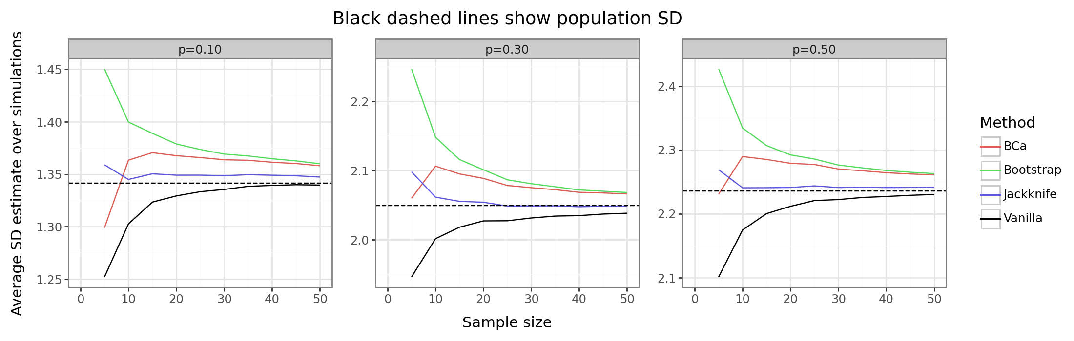
The results above show that the resampling strategies for a bias adjustment are of mixed results. In terms of MAE/MSE, the vanilla method does the best since the resampling strategies introduce additional variance not offset sufficiently (if at all) by the decrease in absolute bias. The second set of figures shows that the jackknife is the best approach for killing the bias quickly. The traditional bootstrap and BCa actually offset by “too much” yielding an overly conservative estimator. The former method actually has a larger absolute bias than the vanilla sample SD.
(3.2) Estimating \(C_n\)
Instead of comparing a measure of linear difference between the bootstrapped and full samples, we could also try to directly estimates \(C_n\) by looking at the distribution of \(S / S^{*}\). We’ll consider three different approaches:
\[\begin{align*} S^{\text{adj}} &= S \cdot C_n^* \\ C_n^* &= \begin{cases} B^{-1} \sum_{i=1}^B \frac{S}{S^*_i} & \text{ average of ratios} \\ \frac{S}{B^{-1} \sum_{i=1}^B S^*_i} & \text{ ratio of averages} \\ \frac{S}{\exp\{B^{-1} \sum_{i=1}^B \log(S^*_i)\}} & \text{ geometric mean} \end{cases} \end{align*}\]I’ve proposed three novel approaches to capturing \(C_n\) through some measure of a ratio statistic. Estimating an unbiased version of a ratio is inherently challenging due to Jensen’s inequality, but this time because it is a convex rather than a concave transformation. Namely, the mean of a ratio will have a positive bias. The ratio of means and geometric mean are two approaches to (hopefully) dilute this bias.
# Loop over each sample size
holder_Cn_binom = []
np.random.seed(seed)
for sample_size in sample_sizes:
    # Draw data
    X = dist_binom.rvs(size=[sample_size, nsim, n_p], random_state=seed)
    # vanilla SD
    sighat_vanilla = X.std(axis=0, ddof=1)
    # bootstrap
    sighat_bs = np.vstack([sd_bs(X[:, idx, :], axis=0, ddof=1, num_boot=B, random_state=seed) for idx in bs_idx])
    sighat_bs_mu = np.mean(sighat_bs, axis=-1)
    # Simple average of ratio
    C_n_bs_mu_ratio = np.mean(np.ma.masked_invalid(np.expand_dims(sighat_vanilla, -1) / sighat_bs), axis=-1)
    # Simple ratio of averages
    C_n_bs_ratio_mu = sighat_vanilla / sighat_bs_mu
    # Average of logs
    C_n_explog = np.exp(np.mean(np.ma.masked_invalid(np.log(np.expand_dims(sighat_vanilla, -1) / sighat_bs)), axis=-1))
    # aggregate results
    di_Cn = di_res = {'vanilla':1,
                    'mu_ratio':C_n_bs_mu_ratio,
                    'ratio_mu': C_n_bs_ratio_mu,
                    'explog': C_n_explog}
    di_Cn = {k:v*sighat_vanilla for k, v in di_res.items()}
    res_Cn = pd.concat(objs=[pd.DataFrame(pd.DataFrame(v, columns=p_seq).assign(method=k)) for k,v in di_Cn.items()])
    res_Cn = res_Cn.melt('method', var_name='p').merge(dat_sd_binom)
    res_Cn = res_Cn.groupby(['method','p']).apply(sim_perf)
    res_Cn = res_Cn.melt(ignore_index=False, var_name='msr').reset_index()
    res_Cn.insert(0, 'n', sample_size)
    del X, di_Cn, sighat_vanilla, sighat_bs, sighat_bs_mu, \
        C_n_bs_mu_ratio, C_n_bs_ratio_mu, C_n_explog
    holder_Cn_binom.append(res_Cn)
# Merge results
res_Cn_binom = pd.concat(holder_Cn_binom)

# Plot the performance
di_method_Cn = {'vanilla':'Vanilla',
                'mu_ratio':'Mean of ratios',
                'ratio_mu': 'Ratio of means',
                'explog': 'Geometric mean'}

# Subset the dat
dat_plot_Cn = res_Cn_binom.query('msr!= "mu"').\
    groupby(['n','method','msr'])['value'].mean().\
        reset_index()

colorz = hue_pal()(3) + ['black']
pn.options.figure_size = (8, 5.5)
gtit = f"SD estimator performance for Bin(m,p)\n$m={m}$, simulations={nsim:,}\nPerformance averaged over three p's: {p_seq}"
gg_perf_Cn_binom = (pn.ggplot(dat_plot_Cn, pn.aes(x='n', y='value', color='method')) +
            pn.theme_bw() + pn.geom_line() + pn.ggtitle(gtit) +
            pn.labs(x = 'Sample size', y='Average measure over simulations') +
            pn.scale_x_continuous(limits=[0, sample_sizes[-1]]) +
            pn.scale_color_manual(name='Method', labels=lambda x: [di_method_Cn[z] for z in x], values=colorz) +
            pn.facet_wrap('~msr', labeller=pn.labeller(cols = lambda x: di_msr[x]), scales='free_y')
            )
gg_perf_Cn_binom

# Plot the actual vs oracle
dat_plot_Cn = res_Cn_binom.query('msr == "mu"').merge(dat_sd_binom)

pn.options.figure_size = (11, 3.5)
gg_Cn_binom = (pn.ggplot(dat_plot_Cn, pn.aes(x='n', y='value', color='method')) +
            pn.theme_bw() + pn.geom_line() +
            pn.facet_wrap(facets='~p', scales='free', labeller=pn.labeller(cols = lambda x: di_p[x])) +
            pn.scale_color_manual(name='Method', labels=lambda x: [di_method_Cn[z] for z in x], values=colorz) +
            pn.geom_hline(pn.aes(yintercept='sd'), data=dat_sd_binom, linetype='--') +
            pn.labs(y='Average SD estimate over simulations', x='Sample size') +
            pn.scale_x_continuous(limits=[0, dat_plot_Cn['n'].max()]) +
            pn.ggtitle('Black dashed lines show population SD'))
gg_Cn_binom
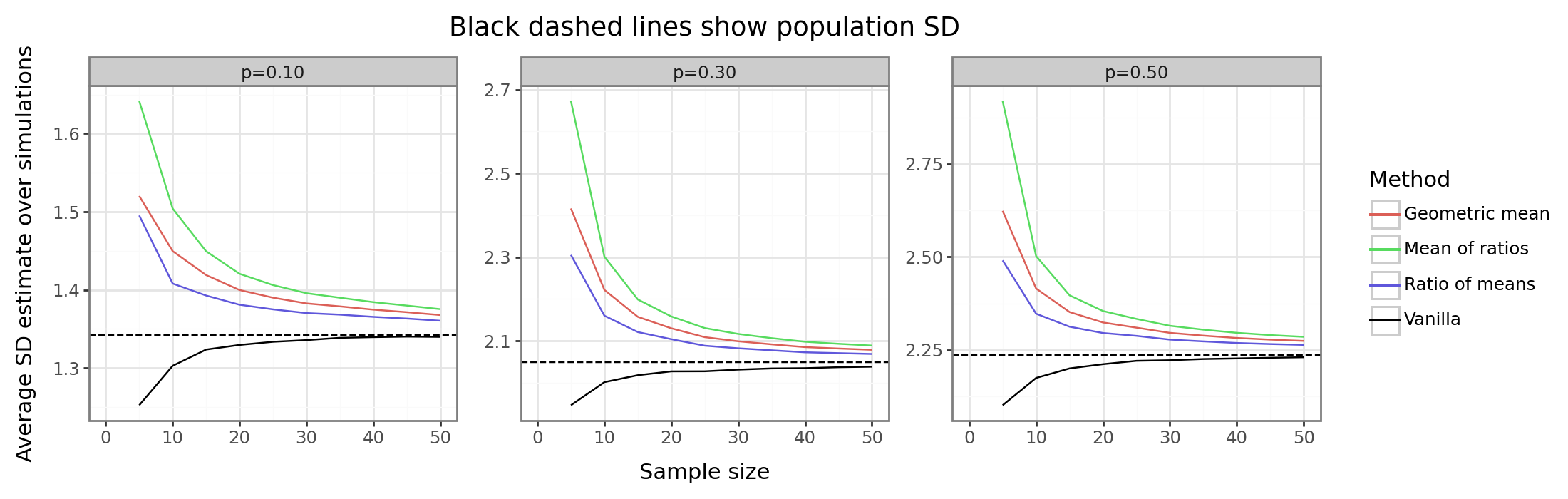
The results above shove that the bootstrapped \(C_n\) estimators are very conservative. Thus, if the goal is to reduce the likelihood of an underestimate of the true SD, then this approach may be useful. But in terms of MAE/MSE, it yields subpar results (at least for this simulation).
(4) Machine learning application
The examples in this post so far have been for known parametric distributions with a single estimable parameter. This has been useful for generating many simulation results quickly and comparing the estimators to the true population parameter. In practice, of course, we will never have a method for knowing the population parameter, and will usually be unaware of the distribution as well. In this final section, we will compare the different estimation strategies we’ve discussed above for estimating the standard deviation of the errors generated by a machine learning (ML) model on a real-world dataset.
ML algorithms are usually evaluated based on different loss metrics such as MSE & MAE (regression), or cross-entropy & accuracy (classification). These metrics are usually simply averages of an error function, and for a given model, these errors have a standard deviation. To formalize notation, consider a learned ML model, \(f_\theta(x): \mathbb{R}^p \to \mathbb{R}\), that maps an input to a scalar (for regression or binary classification), designed to approximate a label \(y\).[8] We are interested in evaluating the model in terms of a loss function: \(\ell(y,f_\theta(x)) = n^{-1} \sum_{i=1}^n \varepsilon(y_i,f_\theta(x_i))\), whose expected value is known as the risk: \(R(f_\theta) = E_{(y,x)\sim P}[\varepsilon(y,f_\theta(x))]\).
In other words, \(\ell\) is an estimator, and \(R\) is a population parameter (conditional on \(f_\theta\)). Like any other statistical estimator, we will often want to know its variance, since this allows us to construct confidence intervals, and predict the number of samples needed to have the standard error be within a certain range and have an associated level of power to reject a null hypothesis. Since we’re only interested in loss functions that are simple averages,[9] the law of large numbers says that \(\sqrt{n}/\sigma_\ell(\ell - R) \to N(0, 1)\), where \(\sigma_\ell = \sqrt{E[\varepsilon-R]^2}\) is the population SD we are interested in estimating.
We will consider the following four error functions: \(\varepsilon(y, f_\theta(x))\), whose average forms some of the most commonly used loss functions in ML.
\[\begin{align*} \varepsilon(y, f_\theta(x)) &= \begin{cases} (y - f_\theta(x))^2 & \text{ for MSE (regression)} \\ |y - f_\theta(x)| & \text{ for MAE (regression)} \\ -[y\log(f_\theta(x)) + (1-y)\log(1-f_\theta(x))] & \text{ for cross-entroy (classification)} \\ I(f_\theta(x) > t = y) & \text{ for accuracy (classification)} \end{cases} \\ E[\varepsilon] &= R(f_\theta), \hspace{3mm} \text{Var}[\varepsilon] = \sigma^2_\ell \end{align*}\]Unless we simulate the data, we won’t know the true data-generating process (DGP), \((y,x)\sim P\). And even if we did know the DGP, we still might know have an analytical form for \(\varepsilon \sim Q\). However, if we use a dataset with sufficiently many held out samples, we can estimate \(R(f_\theta)\) and \(\sigma_\ell\) with close to oracle precision since we know these terms are consistent (and unbiased in the former case), and have a variance that shrinks by \(O(n^{-1})\) due to the law of large numbers.
The California housing dataset will be used since it is has a decent number of observations (~20K) and only 7 features (making it quick to fit). For the regression case, the label is the (log) median housing price, and for the classification case it will be whether the label is above its the median.
The code block below carries out the following simulation. First, 1K training points are randomly sampled to fit an XGBoost model (\(f_\theta\)) with default parameters. Second, the held-out rows (~19K) are used to estimate \(\text{Var}(\varepsilon | f_\theta) = \sigma^2_\ell\). Third, subsets of the held-out data are used to estimate the standard deviation with the different methods discussed in this post. Fourth, the average bias of the different SD estimators is compared to the “oracle” quantity. In effect, we’re comparing how well a sample SD estimator able to randomly sample 10, 15, …, 13177 rows is able to do compared to having access to entire ~19K held-out rows, in terms of bias.
# Load extra modules
import warnings
warnings.filterwarnings('ignore', category=RuntimeWarning)
from time import time
from scipy.stats import uniform
from sklearn.pipeline import Pipeline
from sklearn.preprocessing import StandardScaler
from sklearn.datasets import fetch_california_housing
from sklearn.ensemble import GradientBoostingRegressor, GradientBoostingClassifier

# Load the datasets
X_house, y_house = fetch_california_housing(return_X_y=True)
di_data = {
            'Regression': {'features': X_house,
                          'labels': y_house},
            'Classification': {'features': X_house,
                          'labels': np.where(y_house > np.median(y_house), 1, 0)}
            }

# Define the sample sizes
n = len(X_house)
n_train = 1000
n_test = n - n_train
idx = pd.Series(np.arange(n))
# Fraction of test datapoints to subsample
sd_iter = np.exp(np.linspace(np.log(10), np.log(n_test), 20)).round().astype(int)
print(f'sd_iter = {sd_iter}')

# Initialize the model and preprocessor with default parameters
scaler = StandardScaler()
reg = GradientBoostingRegressor()
clf = GradientBoostingClassifier()
di_mdls = {
            'Regression': Pipeline([('preprocessor', scaler),
                                   ('model', reg)]),
            'Classification': Pipeline([('preprocessor', scaler),
                                   ('model', clf)])
            }

di_resid_fun = {
    'Regression': {
        'MSE': lambda y, f: (y - f)**2,
        'MAE': lambda y, f: np.abs(y - f),
    },
    'Classification': {
        'Accuracy': lambda y, f: np.where(y == np.where(f > 0.5, 1, 0), 1, 0),
        'Cross-Entropy': lambda y, f: -1*(y*np.log(f) + (1-y)*np.log(1-f)),
    }
}

# Increase these later
nsim = 100
n_sd_draw = 100
num_boot = 100
# Generate the sub-sampling index
idx_subsamp = np.argsort(uniform().rvs(size=(n_test, n_sd_draw), random_state=seed), axis=0)

# Run all {nsim} simulations
stime = time()
holder_reg = []
holder_popsd = []
for i in range(nsim):
    # Create the random splits'
    np.random.seed(i+1)
    idx_i = idx.sample(frac=1, replace=False)
    idx_train_i = idx_i[:n_train].values
    idx_test_i = idx_i[n_train:].values
    # Loop over each approach
    for approach, pipe in di_mdls.items():
        print(
                    f'sim = {i+1}\n'
                    f'approach={approach}\n'
                    # f'metric = {metric}\n'
                    # f'num_samp = {n_subsamp}\n'
                )
        # Split the data
        X_train_i = di_data[approach]['features'][idx_train_i]
        y_train_i = di_data[approach]['labels'][idx_train_i]
        X_test_i = di_data[approach]['features'][idx_test_i]
        y_test_i = di_data[approach]['labels'][idx_test_i]
        # Fit the model and get test set prediction
        pipe.fit(X_train_i, y_train_i)
        if hasattr(pipe, 'predict_proba'):
            yhat_test_i = pipe.predict_proba(X_test_i)[:,1]
        else:
            yhat_test_i = pipe.predict(X_test_i)
        # Generate residuals for different loss functions
        for metric, epsilon in di_resid_fun[approach].items():
            # Calculate error functin and "oracle" SD
            resid_i = epsilon(y_test_i, yhat_test_i)
            dat_sd_oracle = pd.DataFrame(
                {'sim':i+1, 'metric':metric, 'approach':approach,
              'oracle':resid_i.std(ddof=1)}, index=[i])
            holder_popsd.append(dat_sd_oracle)
            # Generate sub-sampling index for n_sd_draw random draws
            for n_subsamp in sd_iter[:-1]:
                # Draw residuals from the first {n_subsamp}
                resid_i_subsamp = resid_i[idx_subsamp[:n_subsamp]]
                # (i) Vanilla bootstrap
                sighat_vanilla = np.std(resid_i_subsamp, axis=0, ddof=1)
                # (ii) Kurtosis (adjusted an unadjusted)
                kurtosis_unj = kurtosis(a=resid_i_subsamp, fisher=False, bias=True, axis=0)
                kurtosis_adj = kurtosis(a=resid_i_subsamp, fisher=False, bias=False, axis=0)
                sighat_kurt_unj = sd_adj(x = resid_i_subsamp, kappa=kurtosis_unj, ddof=1, axis=0)
                sighat_kurt_adj = sd_adj(x = resid_i_subsamp, kappa=kurtosis_adj, ddof=1, axis=0)
                # (iii) jackknife (resampling)
                sighat_loo = sd_loo(resid_i_subsamp, axis=0, ddof=1)
                sighat_loo_mu = np.mean(sighat_loo, axis=0)
                bias_jack = (sample_size - 1) * (sighat_loo_mu - sighat_vanilla)
                sighat_jack = sighat_vanilla - bias_jack
                # (iv) bootstrap (resampling)
                sighat_bs = np.vstack([sd_bs(resid_i_subsamp[:,j], axis=0, ddof=1, num_boot=num_boot) for j in range(n_sd_draw)])
                sighat_bs_mu = np.mean(sighat_bs, axis=-1)
                sighat_bs_se = np.std(sighat_bs, axis=-1, ddof=1)
                bias_bs = sighat_bs_mu - sighat_vanilla
                sighat_bs_adj = sighat_vanilla - bias_bs
                # (v) Bias-corrected and accelerated (resampling)
                z0 = np.mean(sighat_bs < np.expand_dims(sighat_vanilla, -1), axis=-1)
                z0 = np.clip(z0, 1/(1+num_boot), None)
                a = moment(sighat_loo, 3, axis=0) / (6 * np.var(sighat_loo, axis=0)**1.5)
                a = np.nan_to_num(a, nan=0)
                bias_bca = z0/(a*z0-1)*sighat_bs_se
                sighat_bca = sighat_vanilla - bias_bca
                # (vi) Mean of ratios (C_n)
                sighat_ratio = np.ma.masked_invalid(np.expand_dims(sighat_vanilla, -1) / sighat_bs)
                Cn_mu_ratio = np.mean(sighat_ratio, axis=-1)
                sighat_mu_ratio = sighat_vanilla * Cn_mu_ratio
                # (vii) ratio of means (C_n)
                Cn_ratio_mu = sighat_vanilla / sighat_bs_mu
                sighat_ratio_mu = sighat_vanilla * Cn_ratio_mu
                # (viii) geometric means (C_n)
                Cn_explog = np.exp(np.mean(np.log(sighat_ratio), axis=-1))
                sighat_explog = sighat_vanilla * Cn_ratio_mu
                # aggregate results
                di_res = {
                    'vanilla': sighat_vanilla,
                    'kurt_unj': sighat_kurt_unj,
                    'kurt_adj': sighat_kurt_adj,
                    'jackknife': sighat_jack,
                    'bootstrap': sighat_bs_adj,
                    'bca': sighat_bca,
                    'mu_ratio': sighat_mu_ratio,
                    'ratio_mu': sighat_ratio_mu,
                    'explog': sighat_explog,
                }
                tmp_res = pd.DataFrame(di_res).\
                    melt(var_name='method', value_name='sd').\
                    assign(sim=i+1, approach=approach, metric=metric, n=n_subsamp)
                holder_reg.append(tmp_res)
                del sighat_vanilla, sighat_kurt_unj, sighat_kurt_adj, sighat_jack, sighat_bs_adj, sighat_bca, sighat_mu_ratio, sighat_ratio_mu, sighat_explog, Cn_mu_ratio, Cn_ratio_mu, Cn_explog, di_res, a, z0, bias_jack, bias_bs, bias_bca, resid_i_subsamp, kurtosis_unj, kurtosis_adj
    # Print time to go
    dtime = time() - stime
    nleft = nsim - (i + 1)
    rate = (i + 1) / dtime
    seta = nleft / rate
    if (i + 1) % 1 == 0:
        print('\n------------\n'
                    f'iterations to go: {nleft} (ETA = {seta:.0f} seconds)\n'
                    '-------------\n')

# Merge results
res_popsd = pd.concat(holder_popsd).reset_index(drop=True)
res_sd_reg = pd.concat(holder_reg).reset_index(drop=True)#.groupby('method').apply(lambda x: x['sd'].isnull().mean()).sort_values()
# Average out over the different lines
res_reg_mu = res_sd_reg.groupby(['method', 'metric', 'approach', 'n', 'sim'])['sd'].mean().reset_index()
# Index to the "full sample" SD
res_reg_mu = res_reg_mu.merge(res_popsd).assign(pct=lambda x: x['sd'] / x['oracle'])
# Calculate average over percent
res_reg_mu = res_reg_mu.groupby(['method', 'metric', 'approach', 'n'])[['sd', 'pct']].mean().reset_index()

# Prepare for plotting
di_method = {
            'vanilla': ['Vanilla', 0],
            'bca': ['BCa', 1],
            'bootstrap': ['Bootstrap', 1],
            'jackknife': ['Jackknife', 1],
            'explog': ['Geometric mean', 2],
            'mu_ratio': ['Mean of ratios', 2],
            'ratio_mu': ['Ratio of means', 2],
            'kurt_adj': ['Adjusted', 3],
            'kurt_unj': ['Unadjusted', 3],
            }

di_type = {
            '0': 'Baseline',
            '1': 'Bias-shift (resampling)',
            '2': 'Bootstrap ($C_n$)',
            '3': 'Kurtosis ($C_n$)',
           }


def di_type_ret(x, di):
    if x in di:
        return di[x]
    else:
        return x

# Tidy up labels
plot_dat = res_reg_mu.assign(category=lambda x: x['method'].map({k:v[1] for k,v in di_method.items()}),
                  method=lambda x: x['method'].map({k:v[0] for k,v in di_method.items()}),
                  )
plot_dat_vanilla = plot_dat.query('method=="Vanilla"').drop(columns=['category','method'])
plot_dat = plot_dat.query('method!="Vanilla"').assign(is_baseline=False)
tmp_dat = plot_dat.groupby(['category','method']).size().reset_index().rename(columns={0:'nrow'})
plot_dat_vanilla = tmp_dat.merge(plot_dat_vanilla.assign(nrow=tmp_dat['nrow'][0])).assign(is_baseline=True)

# Plot the data
def log_labels(breaks):
    return [f"$10^{int(np.log10(x))}$" if x != 1 else "1" for x in breaks]

pn.options.figure_size = (10, 7)
gg_res_mu = (pn.ggplot(plot_dat, pn.aes(x='n', y='pct', color='metric', linetype='is_baseline')) +
             pn.theme_bw() + pn.geom_line() +
             pn.geom_line(data=plot_dat_vanilla) +
             pn.scale_x_log10(labels=log_labels) +
             pn.scale_y_continuous(labels=percent_format()) +
             pn.scale_color_discrete(name='Method') +
             pn.scale_linetype_discrete(name='Baseline (Vanilla)') +
             pn.geom_hline(yintercept=1, linetype='-') +
             pn.facet_wrap('~category+method', ncol=3, scales='free_y', labeller=pn.labeller(cols=lambda x: di_type_ret(x,di_type))) +
             pn.labs(x='Number of test samples', y=f'SD % of n={n_test}') +
             pn.ggtitle(f'Based on average over {nsim} simulations'))
gg_res_mu
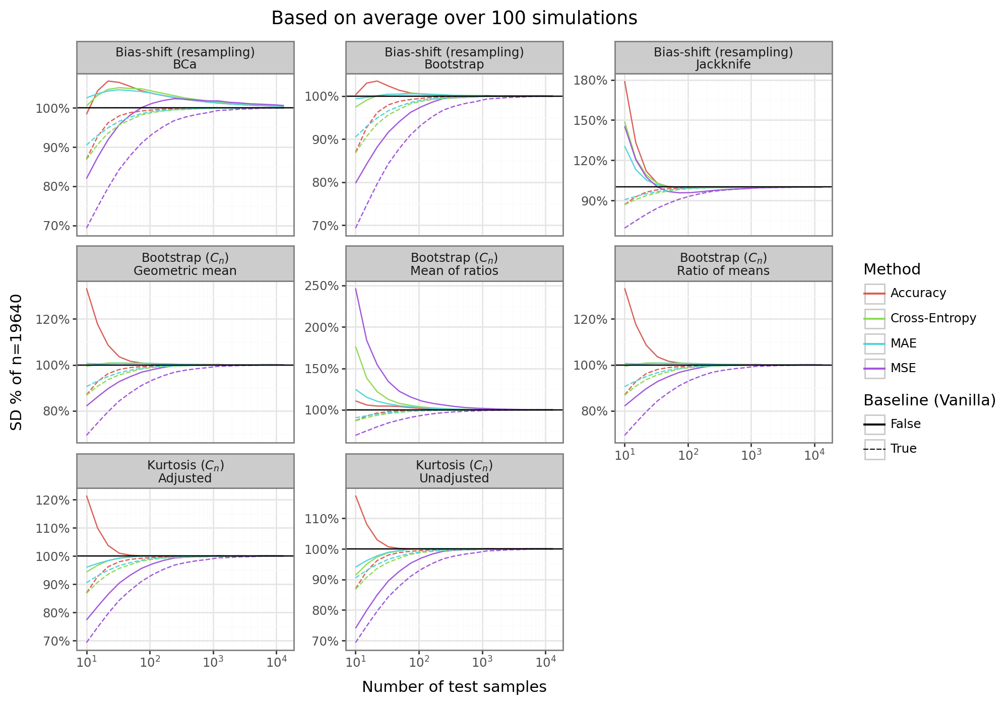
The final figure above shows the SD adjustment results for 8 different estimators across four different loss/error metrics benchmarked against the baseline vanilla sample SD estimator. All of the estimators are less negatively biased than the baseline approach, and sometimes have an absolute bias that is improved as well. For most of the metrics, the bias of the baseline SD estimator disappears by around 100 samples. However, for the MSE loss function/error, at least 1000 samples are needed to kill the bias. In contrast, some of the adjustment methods are able to kill the bias by 10 samples, and the MSE by 100 samples.
For the \(C_n\)-kurtosis estimators, the bias tends to be negative, but less severe (except for the accuracy error/loss which has a positive bias). For the resampling bias-shifts, the bootstrap sometimes biases high, and other times biases low. Furthermore the bias is not always monotonically decreasing, even if it is asymptotically vanishing, making the results harder to characterize. The other resampling technique, the jackknife, produces consistently conservative estimates, although these are not, in absolute terms, smaller than the baseline estimator. For the bootstrapped \(C_n\)-approaches, the mean of ratios is the most conservative, and significantly biased. In contrast, the geometric mean tends to do much better at killing the bias quickly, especially compared the vanilla estimator.
Overall, there are trade-offs for different estimators. In terms of reducing the absolute bias, the normal bias-offset bootstrap, or the geometric mean for the adjustment factor works well. For a reliably conservative estimator, the jackknife is best suited.
(5) Conclusion and other directions
This post has has provided a thorough and up-to-date overview of what causes the traditional SD estimator to be biased, and methods to help de-bias it. A variety of parametric simulations demonstrated quality of different adjustment procedures. For these toy examples, the bias adjustment methods tended to work quite well, especially the “plug-and-play” estimator for a known parametric form. In the real-world, unfortunately, such an approach is likely infeasible since we almost never know the actual data distribution.
To highlight the challenge of estimating the sample SD on real-world data, we examined the sample SD on four different “errors” generated by a ML algorithm for four standard loss functions. A total of eight different adjustment procedures were considered including those using first-order adjustments (i.e. the kurtosis estimators), resampling methods to estimate the bias offset (i.e. bootstrap and jackknife), and resampling methods to estimate the adjustment factor directly.
On this real-world data, the bias of the vanilla sample SD could be persistent and noticeable up to 1000 samples. In contrast, many of the adjustment approaches were able to kill the bias much faster. However, the direction and magnitude of the bias was not always predictable. Specifically, some methods could obtain conservative estimates of the sample SD (i.e. a positive bias), but have larger absolute errors. In contrast, others had lower absolute bias, but varied in the direction the bias could take.
In summary, there is no “right” approach for adjusting the sample SD bias. For practitioners who need to adjust the bias from the negative to the positive direction, the jackknife is the clear way to go. When the goal is to minimize the absolute bias, the traditional bootstrap bias-shift is likely the most effective. If the goal is to minimize the bias for very small sample sizes, then using the geometric mean of the resampled ratios could instead be the most efficacious.
As a final note, I also did some preliminary investigations into directly estimating \(C_n\) through optimization routines (see this script). Namely, by subsampling from a draw of data (like the delete-k jackknife), we can observe: \([S_{2}, S_{3}, \dots, S_{n} ]\), where \(S_{i}\) is the average sample SD for \(i\) observations. With these observations in hand, we can fit one of two non-linear regression models.
First, since \(S_{i} \approx \frac{\sigma}{C_i}\), define \(C_i = 1 + \frac{\beta}{i^\gamma}\), where we now try to learn \((\sigma, \alpha, \beta, \gamma)\) directly. Second, we can obviate the need to learn \(\sigma \) directly, by considering the ratio of \(S_{i} / S_{j} \approx (j/i)^{\gamma}(\frac{i^\gamma + \beta}{j^\gamma + \beta}) \). Now having learned a new \(C_n \) function we can directly predict \( \sigma \) for any estimated \( S \), which has some known sample size. Unfortunately, my initial exploration into these direct optimization frameworks yielded unsatisfying results. However, it may be that additional experimentation and optimization procedures could yield improved results. These two approaches are, as far as I know, unexplored.
References
-
And if the data is Gaussian, the sample variance actually has a chi-squared distribution and therefore exact confidence intervals can be generated. ↩
-
Note that an alternative formulation a la Cureton (1968) is to re-write the sample SD as \(S = \sqrt{\sum_i (X_i \bar{X})^2 / k_n}\) so that we have a different adjustment factor than the usual Bessel Correction. ↩
-
As in, if \(n\) is very large, like \(n=1e8\) vs \(n=2e8\), then the SE reduction will be close to exact. ↩
-
Note that the “adjusted” approach yields an unbiased estimator in the case of a normal distribution. ↩
-
It’s possible that the kurtosis of a distribution is a function of population parameters for which there is no MLE estimator, or of parameters whose best for estimators have poor poor statistical qualities. For example, if the upper/lower bound of a truncated Gaussian need to be estimated, it may be that these parameters are significantly biased or not even consistent. ↩
-
Unless the parametric form is known, in which case the adjusted non-parametric method should not be considered. ↩
-
To see why this is the case, imagine drawing 100 million samples from an exponential distribution. The average of 100 million data points will be very same, no matter “which” 100 million data points were draw. In contrast, if you draw two data points from an exponential distribution, the average will vary wildly because there’s a good chance you’ll draw two small numbers, two large numbers, a large and a small number, etc. ↩
-
For multitask or multiclass classification, the model will instead map \(f_\theta(x): \mathbb{R}^p \to \mathbb{R}^k\), but we can still often reduce the loss function to a single value. ↩
-
There are other loss functions used in ML like precision or concordance which are not simple averages since the \(i^{th}\) and \(j^{th}\) error are not independent of each other. ↩