In this post I describe how to calculate the first and second moments of a loss function for a machine learning (ML) model. The expected value of a loss function is known as its risk, and I refer to the second central moment as the loss variance. While these quantities are not perfectly knowable in the real world, in the simulation setting the researcher has full knowledge of how data is generated and can therefore calculate them in principle. But how does one do this for an arbitrary distribution and loss function? That is the question this post will answer.

Three strategies are covered: Monte Carlo integration (MCI), trapezoidal numerical integration, and double quadrature. Each strategy can be applied to either a joint distribution over \((Y, X)\) or a conditional distribution \(Y \vert X\) combined with a marginal distribution for \(X\). As a regression benchmark, both the Gaussian case (where closed-form expressions exist) and non-Gaussian noise (where only numerical methods apply) are considered. The post concludes with a classification example covering log-loss and the 0/1 accuracy loss.

The rest of this post is structured as follows. Section 1 provides background on the supervised ML problem and the integration approaches used. Section 2 works through three regression scenarios of increasing complexity. Section 3 covers classification. Section 4 concludes.

For readability, various code blocks have been suppressed and the text has been tidied up. All figures are produced by this script.

(1) Background

(1.1) The ML problem

The goal of supervised machine learning is to “learn” a function \(f_\theta(x)\), \(f: \mathbb{R}^p \to \mathbb{R}^k\), that maps a feature vector \(x \in \mathbb{R}^p\) and seeks to approximate a label \(y\). We assume that the actual data generating process (DGP) follows some (unknown) probabilistic joint distribution \(P_{\phi}(Y,X)\). In a supervised learning scenario we have a dataset \( \{(y_i, x_i)\}^n_{i=1} \) consisting of \(n\) observations. We learn \(\theta\) by minimizing some training loss: \(\hat\theta = \arg\min_\theta \hat\ell(y, f_\theta(x))\). Once training is complete, \(f_{\hat\theta}\) hopefully generalizes to new data drawn from \(P_\phi\).

After a model is trained, we are often interested in how well it will perform on future data for some primary loss function \(\ell\).[¹] The expected value of this loss is the risk:

We may also be interested in the variance of the loss:

The loss variance is less commonly discussed than the risk, but its main use is in understanding how quickly the empirical risk converges to the true risk. By the central limit theorem, \(\sqrt{n}(\hat{R} - R) \to N(0,V(\theta))\) asymptotically, so the loss variance directly governs the width of confidence intervals for \(R\).

(1.2) The integration problem

(1.2.1) Joint integration approach

If one knows the true DGP, the risk is in principle solvable as a double integral:

where \(p(\cdot)\) denotes the joint density.[²] Similarly, the loss variance requires computing:

In other words, once the risk is known, computing the loss variance only requires integrating the squared loss function over the joint distribution.

(1.2.2) Conditional integration approach

If we know the unconditional distribution of \(X\) and the conditional distribution of \(Y \vert X\), the law of total expectation lets us rewrite the risk as:

Since we often think of the covariates as “causing” the labels, this is frequently a more natural decomposition. It also has practical advantages: the joint distribution \(p(y,x)\) may be difficult to characterize analytically even when \(p_X(x)\) and \(p_{Y \vert X}(y \vert x)\) are both tractable.[³]

(1.3) Monte Carlo integration

If a researcher can draw from the joint or conditional distribution, the simplest approach is Monte Carlo integration (MCI). Its precision is controlled entirely by sample size.

Joint sampling

1. Draw \(n\) samples \(\{(y_i, x_i)\}^n_{i=1}\) with \((y_i, x_i) \sim P_{Y,X}\)
2. Evaluate \(\ell_i = \ell(y_i, f_\theta(x_i))\)
3. Estimate \(\hat{R} = n^{-1}\sum_{i=1}^n \ell_i\) and \(\hat{V} = (n-1)^{-1}\sum_{i=1}^n \ell_i^2 - [\hat{R}]^2\)

Conditional sampling

1. Draw \(x_i \sim P_X\)
2. Draw \(y_i \vert x_i \sim P_{Y \vert X}\)
3. Proceed as above

(1.4) Numerical methods

Unlike MCI, numerical methods are deterministic and can be run to a specified tolerance, but they require knowing the density function. Throughout this post I use the trapezoidal rule: \(\int_a^b f(x) dx \approx \sum_{i=2}^{n} \frac{f(x_{i})+f(x_{i-1})}{2}(x_i - x_{i-1})\). For a two-dimensional integral the steps are:

Joint density

1. Discretize onto a grid \(\hat{\mathcal{X}} = {x_1,\ldots,x_{n_x}}\) and \(\hat{\mathcal{Y}} = {y_1,\ldots,y_{n_y}}\)
2. For each \(x_i\), compute the inner integral: \(I(x_i) = \text{trapz}\big(\ell(y, f_\theta(x_i)) \cdot p(y, x_i),\; y \in \hat{\mathcal{Y}}\big)\)
3. Compute the outer integral: \(\hat{R} = \text{trapz}\big(I(x),\; x \in \hat{\mathcal{X}}\big)\)

Conditional density

Steps (1) and (2) differ only in that the inner integral uses \(p_{Y \vert X}(y, X{=}x_i)\) and the outer integral weights by \(p_X(x)\):

For the loss variance, one computes the same integral with \(\ell^2\) in place of \(\ell\), then subtracts \([\hat{R}]^2\).

The trapezoidal approach trades off grid resolution (\(n_y, n_x\)) against accuracy, and scales as \(O(n_y \cdot n_x)\) operations. I also compare against double Gaussian quadrature (scipy.integrate.dblquad) in the worked example. Compared to MCI, numerical methods are more precise for low-dimensional, smooth integrands, but become impractical as the dimensionality of \(X\) grows.

(1.5) Worked example

To ground the three integration strategies in a concrete example, consider a bivariate normal (BVN) DGP, \((Y, X) \sim \text{BVN}(\mu, \Sigma)\), with the following custom loss function:

This loss has no closed-form risk or variance — there is no analytic expression for \(\int\int \|y\| \log(x^2) \, p(y,x) \, dy\, dx\) under the BVN density — making it a useful benchmark for comparing the numerical methods. All three strategies (MCI, trapezoidal, and double quadrature) should converge to the same value; agreement across methods serves as a mutual validation.

For the conditional approach, the BVN has the convenient property that \(Y \vert X{=}x\) is Gaussian with a known mean and variance:

so the conditional distribution is available analytically. This is encapsulated in the dist_Ycond_BVN helper class.

All three integration strategies are implemented in a small library with two classes: MonteCarloIntegration and NumericalIntegrator. Both accept a loss function of the form loss(y=..., x=...) and either a joint distribution (dist_joint) or a pair of conditional and marginal distributions (dist_Y_condX, dist_X_uncond). The full source for these utilities is available in the _rmd/extra_loss_moments/ folder of the GitHub repo.

import numpy as np
from scipy.stats import norm, multivariate_normal
from _rmd.extra_loss_moments.utils import dist_Ycond_BVN
from _rmd.extra_loss_moments.MCI import MonteCarloIntegration
from _rmd.extra_loss_moments.trapz import NumericalIntegrator

# BVN parameters
mu_Y, mu_X   = 2.4, -3.5
sigma_Y, sigma_X = np.sqrt(2.1), np.sqrt(0.9)
rho = 0.7
cov = [[sigma_Y**2, rho*sigma_Y*sigma_X],
       [rho*sigma_Y*sigma_X, sigma_X**2]]

dist_YX = multivariate_normal(mean=[mu_Y, mu_X], cov=cov)
dist_X  = norm(loc=mu_X, scale=sigma_X)
dist_Yx = dist_Ycond_BVN(mu_Y=mu_Y, sigma_Y=sigma_Y,
                          sigma_X=sigma_X, rho=rho, mu_X=mu_X)

# A custom loss function
def loss_custom(y, x):
    return np.abs(y) * np.log(x**2)

mci_joint  = MonteCarloIntegration(loss=loss_custom, dist_joint=dist_YX)
mci_cond   = MonteCarloIntegration(loss=loss_custom,
                                    dist_X_uncond=dist_X, dist_Y_condX=dist_Yx)
ni_joint   = NumericalIntegrator(loss=loss_custom, dist_joint=dist_YX)
ni_cond    = NumericalIntegrator(loss=loss_custom,
                                  dist_X_uncond=dist_X, dist_Y_condX=dist_Yx)

The code block below shows how to call each estimator and recover both the risk and loss variance.

# MCI – joint and conditional
risk_mci_j, var_mci_j = mci_joint.integrate(
    num_samples=500_000, seed=1234, calc_variance=True)
risk_mci_c, var_mci_c = mci_cond.integrate(
    num_samples=500_000, seed=1234, calc_variance=True)

# Numerical – quadrature and trapezoidal (joint), trapezoidal (conditional)
risk_jq, var_jq = ni_joint.integrate(
    method='quadrature', calc_variance=True, k_sd=5, sol_tol=1e-3)
risk_jt, var_jt = ni_joint.integrate(
    method='trapz_loop', calc_variance=True, k_sd=5, n_Y=200, n_X=201)
risk_ct, var_ct = ni_cond.integrate(
    method='trapz_loop', calc_variance=True, k_sd=5, n_Y=200, n_X=201)

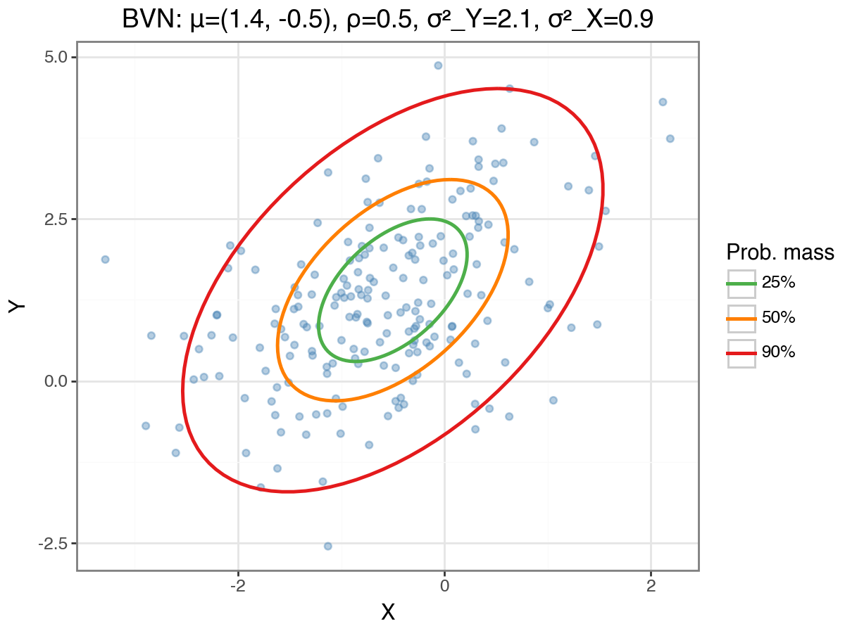
The bivariate normal (BVN) distribution used in this example is illustrated below. The coloured ellipses trace the 25%, 50%, and 90% probability mass contours; these are obtained by Cholesky-decomposing the covariance matrix and scaling the parametric unit circle by the appropriate chi-squared quantile.

All five integration strategies produce nearly identical estimates for both the risk and the loss variance, as shown in Figure 2. The dashed horizontal line is a high-precision reference computed from five million MCI samples.

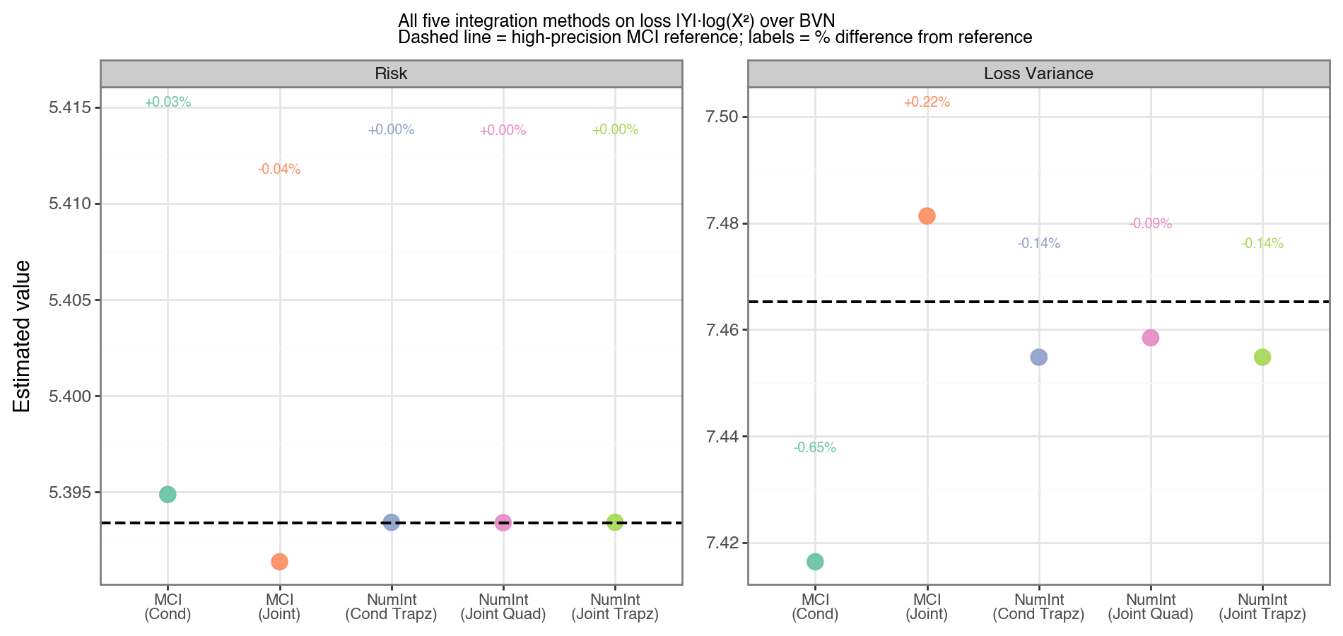
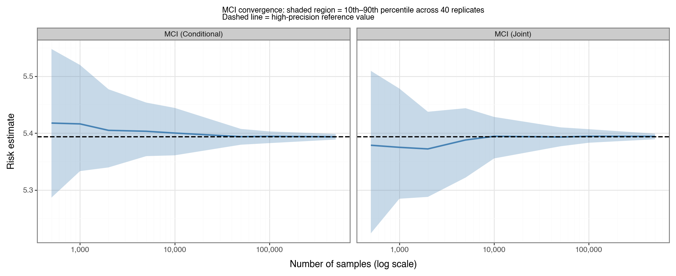
Figure 3 illustrates how the MCI risk estimate converges to the true value as the sample size grows, shown separately for joint and conditional sampling. The shaded band is the 10th–90th percentile spread across 40 independent replicates. Even at \(n=500\), the estimate is in the right ballpark; at \(n=10{,}000\) the spread is already narrow. However, to ensure the estimation variation is produced <1% error most of the time, 100K draws are required.

(2) Regression models

For each scenario I use a linear model \(f_\theta(x) = \theta_0 + \theta_1 x\). To isolate the effect of the slope \(\theta_1\), I always set the intercept to its conditionally optimal value: \(\theta_0 = \mu_Y - \theta_1 \mu_X\), which ensures that \(E[Y - f_\theta(X)] = 0\). With this convention, varying \(\theta_1\) controls only the bias-variance trade-off in the slope.

The BVN parameters used throughout Section 2 are \(\mu_Y=2\), \(\mu_X=1.5\), \(\sigma_Y^2=3\), \(\sigma_X^2=1.5\), and \(\rho=0.6\).

(2.1) Squared loss, Gaussian covariates

Setup and closed-form risk

Consider \((Y, X) \sim \text{BVN}(\mu, \Sigma)\) and squared loss \(\ell(y, \hat{y}) = (y - \hat{y})^2\). Define the residual \(Z = Y - \theta_0 - \theta_1 X\). Since \(Z\) is a linear combination of jointly Gaussian random variables, it is itself Gaussian:

The risk is then simply the second moment of \(Z\). This follows from the standard identity \(E[Z^2] = \text{Var}(Z) + (E[Z])^2\), which holds for any random variable:

Minimising over \((\theta_0, \theta_1)\) gives the ordinary-least-squares solution. With the parameterization above (\(\theta_0\) always set optimally), the slope optimum is \(\theta_1^* = \rho \sigma_Y / \sigma_X\), which sets \(\mu_Z = 0\) and minimises \(\sigma_Z^2\) simultaneously. Substituting \(\theta_0^\) and \(\theta_1^\) into \(R(\theta)\) gives the minimum risk — the irreducible noise that cannot be explained by any linear function of \(X\):

This has an intuitive interpretation. When \(\rho = 1\), \(X\) and \(Y\) are perfectly linearly related, so knowing \(X\) determines \(Y\) exactly and \(R^* = 0\). When \(\rho < 1\), there is variance in \(Y\) that is orthogonal to \(X\) — i.e. noise that no linear predictor can capture — and \(R^*\) is that irreducible component. In fact, \(1 - \rho^2\) is exactly one minus the coefficient of determination \(R^2 = \rho^2\) from a simple linear regression of \(Y\) on \(X\).

Closed-form loss variance

Because \(Z \sim N(\mu_Z, \sigma_Z^2)\) and \(\ell = Z^2\), the loss variance only requires the fourth moment of a normal random variable. Using \(E[Z^4] = 3\sigma_Z^4 + 6\mu_Z^2\sigma_Z^2 + \mu_Z^4\):

At the optimum where \(\mu_Z = 0\), the loss variance simplifies to \(V^* = 2[\sigma_Y^2(1-\rho^2)]^2 = 2(R^*)^2\), a well-known result for the variance of a chi-squared (one degree of freedom) scaled random variable.

Implementation and validation

# Analytical closed forms
def risk_sq_closed(theta0, theta1, mu_Y, mu_X, sigma_Y, sigma_X, rho):
    mu_Z  = mu_Y - theta0 - theta1*mu_X
    var_Z = sigma_Y**2 - 2*theta1*rho*sigma_Y*sigma_X + theta1**2*sigma_X**2
    return mu_Z**2 + var_Z

def var_sq_closed(theta0, theta1, mu_Y, mu_X, sigma_Y, sigma_X, rho):
    mu_Z  = mu_Y - theta0 - theta1*mu_X
    var_Z = sigma_Y**2 - 2*theta1*rho*sigma_Y*sigma_X + theta1**2*sigma_X**2
    return 2*var_Z**2 + 4*mu_Z**2*var_Z

# Validate with numerical methods at a single theta_1
theta1_opt = rho * sigma_Y / sigma_X  # = 0.6 * sqrt(3) / sqrt(1.5) ≈ 0.849
theta0_opt = mu_Y - theta1_opt * mu_X

def loss_sq(y, x):
    return (y - theta0_opt - theta1_opt*x)**2

mci = MonteCarloIntegration(loss=loss_sq, dist_joint=dist_YX_reg)
ni  = NumericalIntegrator(loss=loss_sq,  dist_joint=dist_YX_reg)

risk_mci, var_mci   = mci.integrate(num_samples=500_000, seed=1234, calc_variance=True)
risk_trapz, var_trapz = ni.integrate(method='trapz_loop', calc_variance=True,
                                      k_sd=5, n_Y=150, n_X=151)
risk_exact = risk_sq_closed(theta0_opt, theta1_opt, mu_Y, mu_X, sigma_Y, sigma_X, rho)

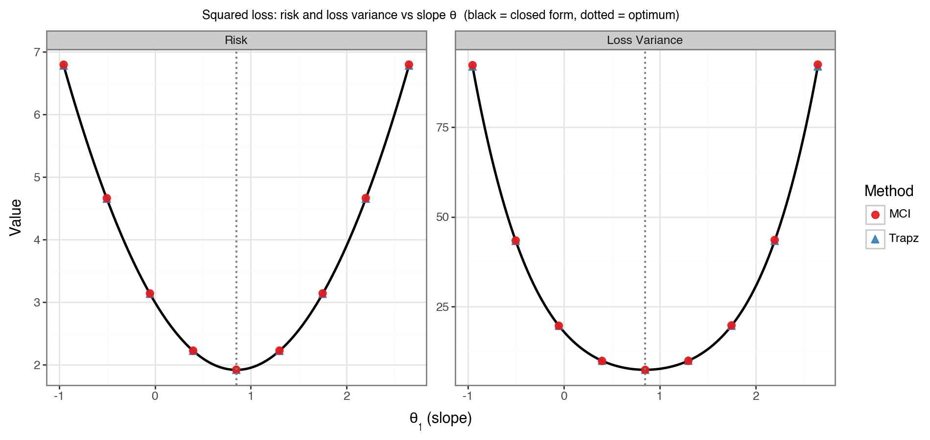
Figure 4 plots both the risk and loss variance as functions of \(\theta_1\) across a \(\pm 1.8\) window around the optimum. The black line is the closed-form expression; red dots are MCI estimates; blue dots are trapezoidal estimates. All three agree closely across the full range. The dotted vertical line marks \(\theta_1^*\), confirming that the risk is indeed minimised there.

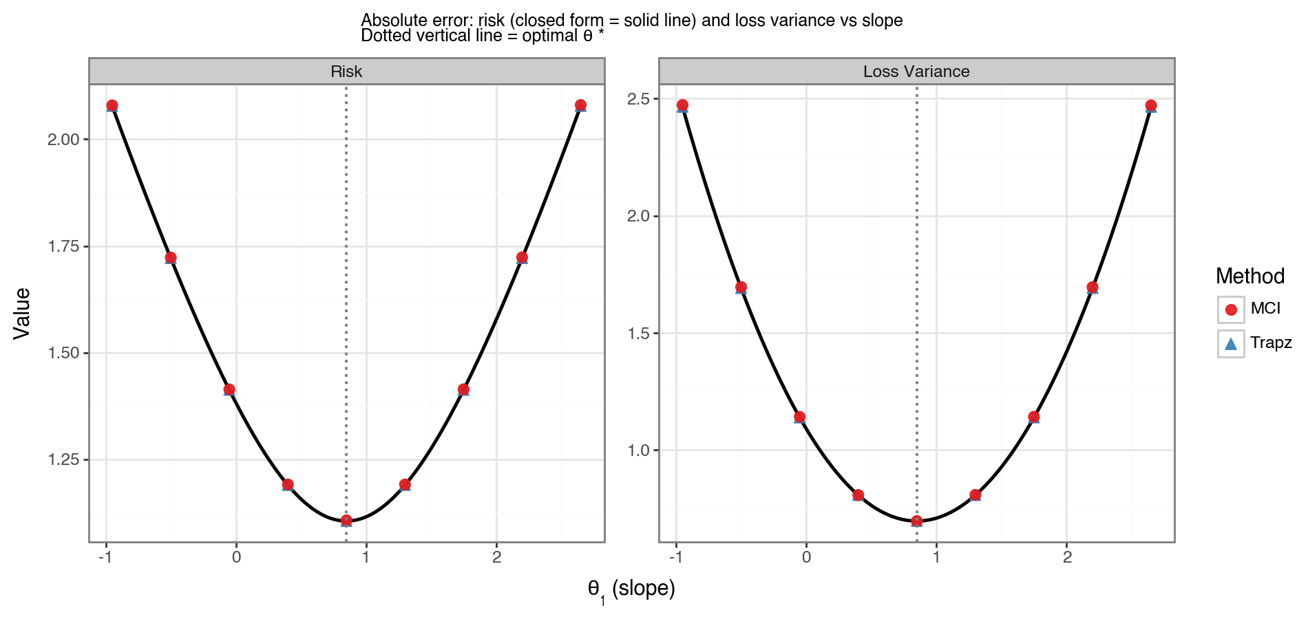
(2.2) Absolute error, Gaussian covariates

Replacing squared loss with absolute error, \(\ell(y, \hat{y}) = \|y - \hat{y}\|\), the risk becomes \(R(\theta) = E[\|Z\|]\) where \(Z \sim N(\mu_Z, \sigma_Z^2)\) as before. The expected absolute value of a Gaussian random variable has an exact formula:[⁴]

The loss variance for absolute error has a surprisingly clean form. Since \(\|Z\|^2 = Z^2\) always:

This is simply the variance of the half-normal (or folded-normal) distribution.

from scipy.stats import norm as _norm

def risk_abs_closed(theta0, theta1, mu_Y, mu_X, sigma_Y, sigma_X, rho):
    mu_Z    = mu_Y - theta0 - theta1*mu_X
    sigma_Z = np.sqrt(sigma_Y**2 - 2*theta1*rho*sigma_Y*sigma_X + theta1**2*sigma_X**2)
    return (sigma_Z * np.sqrt(2/np.pi) * np.exp(-mu_Z**2 / (2*sigma_Z**2))
            + mu_Z * (1 - 2*_norm.cdf(-mu_Z/sigma_Z)))

def var_abs_closed(theta0, theta1, mu_Y, mu_X, sigma_Y, sigma_X, rho):
    mu_Z  = mu_Y - theta0 - theta1*mu_X
    var_Z = sigma_Y**2 - 2*theta1*rho*sigma_Y*sigma_X + theta1**2*sigma_X**2
    r     = risk_abs_closed(theta0, theta1, mu_Y, mu_X, sigma_Y, sigma_X, rho)
    return mu_Z**2 + var_Z - r**2

Figure 5 shows the resulting risk and loss variance curves. The shape is qualitatively similar to Figure 4, except that absolute error is less sensitive to the tails of \(Z\) and therefore has a shallower curvature. The numerical estimates (MCI and trapezoidal) again agree with the closed-form curves.

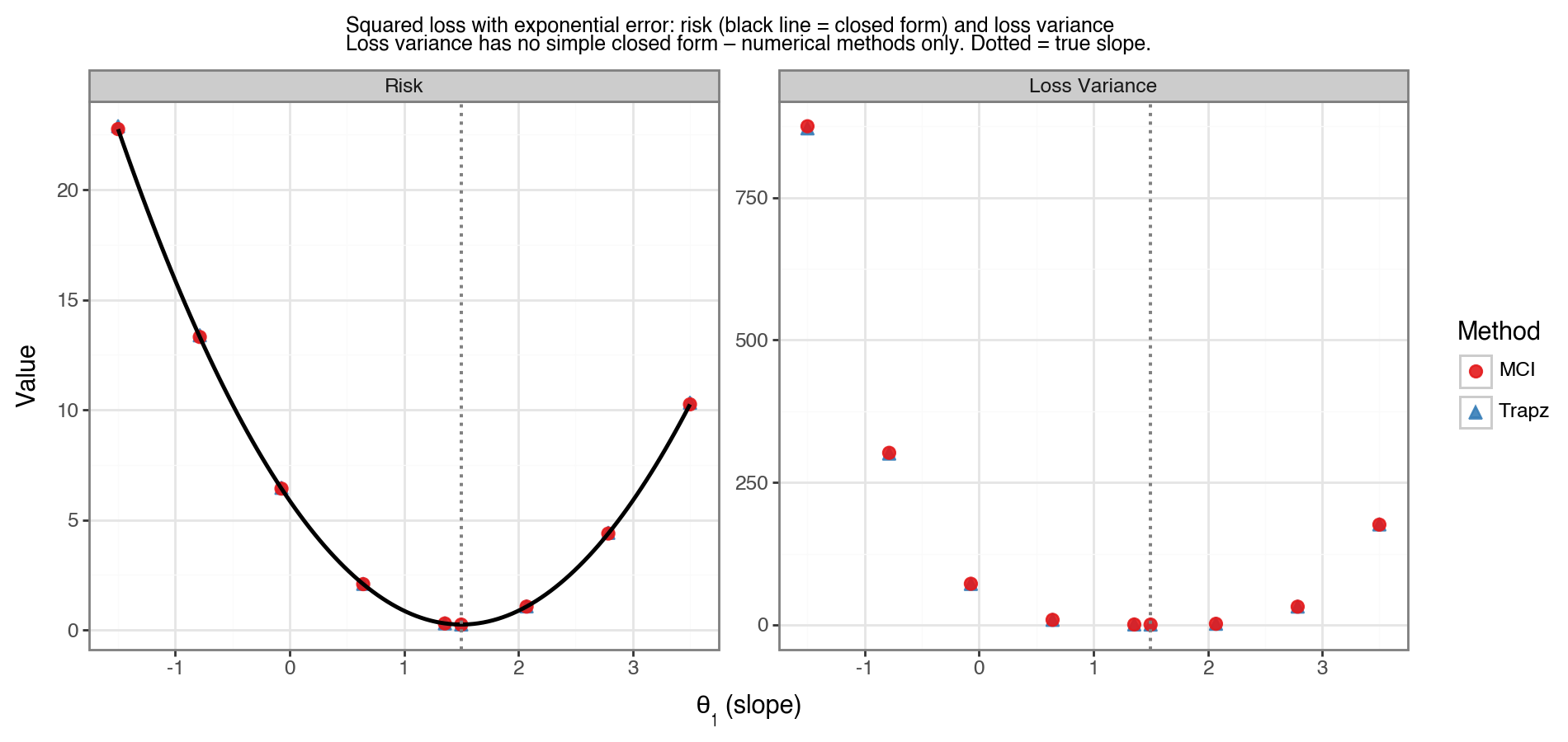
(2.3) Squared loss, non-Gaussian error

The Gaussian assumption in Sections 2.1–2.2 is convenient but not always realistic. What happens to the moments when the error distribution is non-Gaussian? To make this concrete, consider:

Subtracting \(\lambda^{-1}\) ensures \(E[\varepsilon - \lambda^{-1}] = 0\), so \(E[Y \vert X{=}x] = \alpha + \beta x\). Let \(\eta = \varepsilon - \lambda^{-1}\) denote the mean-zero exponential noise, with \(\text{Var}(\eta) = \lambda^{-2}\).

Risk

With squared loss and model \(f_\theta(x) = \theta_0 + \theta_1 x\), the residual is \(Z = (a + bX) + \eta\) where \(a = \alpha - \theta_0\) and \(b = \beta - \theta_1\). Since \(\eta \perp X\):

The formula is structurally identical to the Gaussian case in Section 2.1, with the noise variance term \(\lambda^{-2}\) simply added on. The optimal slope remains \(\theta_1^* = \beta\) and the minimum risk is \(R^* = \lambda^{-2}\).

Loss variance

The loss variance is more involved. Because \(Z\) is now a sum of a Gaussian term \((a+bX)\) and a skewed term \(\eta\), the distribution of \(Z\) is asymmetric and its fourth moment mixes cumulants from both components. While a closed-form expression exists via the cumulant generating function, it is not a compact formula and offers little intuition. This is precisely the scenario where numerical integration — MCI or the trapezoidal rule applied to the conditional distribution \(Y \vert X\) — is most valuable.

from scipy.stats import expon

class dist_Ycond_LinearExp:
    """Y | X=x ~ ShiftedExp: loc = alpha + beta*x - 1/rate"""
    def __init__(self, alpha, beta, rate):
        self.alpha, self.beta, self.rate = alpha, beta, rate

    def __call__(self, x):
        loc = self.alpha + self.beta*np.asarray(x) - 1.0/self.rate
        return expon(loc=loc, scale=1.0/self.rate)

alpha_true, beta_true, rate = 0.5, 1.5, 2.0
dist_X_ng   = norm(loc=1.0, scale=np.sqrt(1.5))
dist_Yx_ng  = dist_Ycond_LinearExp(alpha=alpha_true, beta=beta_true, rate=rate)

def loss_sq_t0(t0, t1):
    def _loss(y, x): return (y - t0 - t1*x)**2
    return _loss

ni_ng = NumericalIntegrator(loss=loss_sq_t0(alpha_true, 1.0),
                             dist_X_uncond=dist_X_ng, dist_Y_condX=dist_Yx_ng)
risk_ng, var_ng = ni_ng.integrate(method='trapz_loop', calc_variance=True,
                                   k_sd=6, n_Y=150, n_X=151)

Figure 6 shows the risk and loss variance as a function of \(\theta_1\) for this model. For the risk (left panel), the solid black line is the closed-form expression; MCI and trapezoidal estimates match it closely. For the loss variance (right panel), no black line is shown because no compact closed-form expression is used — both numerical methods serve as the reference, and they agree with each other. The minimum risk is at the true slope (dotted vertical line), and the loss variance is largest where the model is most misspecified.

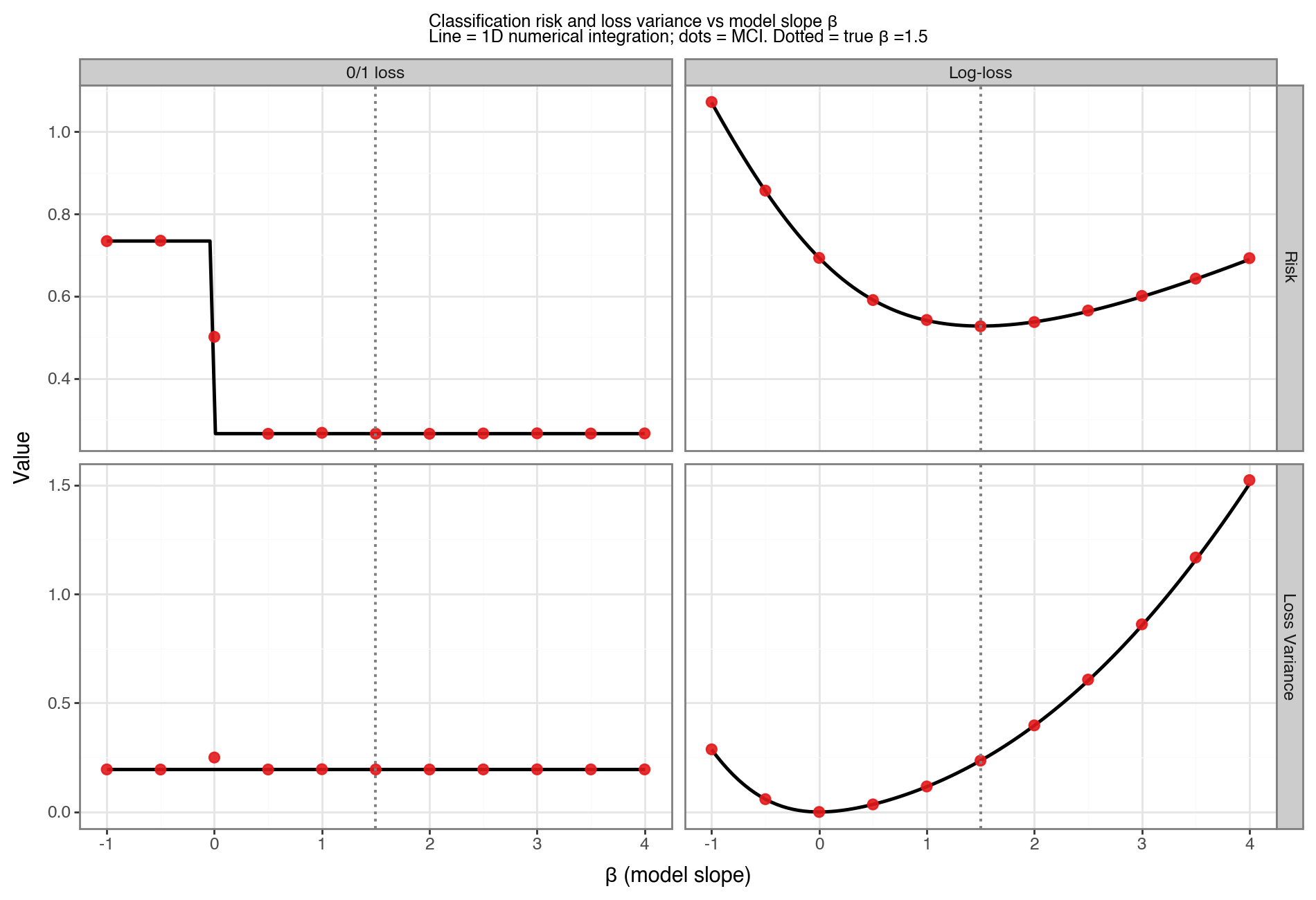
(3) Classification models

In classification, \(Y \in {0, 1}\) is a binary label. The conditional distribution \(Y \vert X\) is Bernoulli rather than Gaussian, so the NumericalIntegrator class (which integrates over a continuous \(Y\) grid) does not apply directly. Instead, we use two complementary approaches: MCI (which works for any distribution) and a one-dimensional numerical integral over \(X\) alone (exploiting the fact that the inner integral over \(Y\) can be computed analytically for each \(x\)).

The setup throughout is:

• \(X \sim N(0, 1)\)
• True DGP: \(P(Y{=}1 \vert X{=}x) = \sigma(\beta_0 x)\) where \(\sigma\) is the logistic function and \(\beta_0 = 1.5\)
• Model: \(\hat{P}(Y{=}1 \vert X{=}x) = \sigma(\beta x)\) for varying \(\beta\)

Using the law of total expectation, the risk reduces to a one-dimensional integral:

where \(g(x;\beta) = E[\ell(Y, f_\beta(x)) \vert X{=}x]\) is a deterministic function of \(x\) that depends on both the loss function and the model. This 1D integral is easy to compute with numpy.trapz, and the loss variance follows from \(V = \int g^{(2)}(x;\beta) f_X(x)\, dx - R^2\) where \(g^{(2)}\) replaces \(\ell\) with \(\ell^2\) in the conditional expectation.

(3.1) Log-loss

The log-loss (or binary cross-entropy) is:

For a given \(x\), the conditional expected log-loss is:

where \(p(x) = \sigma(\beta_0 x)\) is the true success probability. The risk is minimised when \(\beta = \beta_0\) (perfectly specified model), where it equals the entropy of the outcome distribution averaged over \(X\).

CLIP = 1e-10

def sigmoid(x):
    return 1.0 / (1.0 + np.exp(-np.asarray(x, dtype=float)))

def p_true(x, beta0=1.5):
    return sigmoid(beta0 * x)

def log_loss_cond_exp(x, beta, power=1):
    """E[L^power | X=x] for log-loss."""
    p    = p_true(x)
    phat = np.clip(sigmoid(beta * x), CLIP, 1 - CLIP)
    l1   = -np.log(phat)
    l0   = -np.log(1.0 - phat)
    return p * l1**power + (1.0 - p) * l0**power

def numint_1d_clf(cond_fn, cond2_fn, k_sd=5, n_X=400):
    """1D trapezoidal integration over X for classification risk and variance."""
    xvals = np.linspace(-k_sd, k_sd, n_X)
    fX    = norm.pdf(xvals)
    risk  = np.trapz(cond_fn(xvals) * fX, xvals)
    risk2 = np.trapz(cond2_fn(xvals) * fX, xvals)
    return risk, risk2 - risk**2

# Risk and variance for a single beta value
beta_test = 1.0
risk_ll, var_ll = numint_1d_clf(
    cond_fn =lambda x: log_loss_cond_exp(x, beta_test, power=1),
    cond2_fn=lambda x: log_loss_cond_exp(x, beta_test, power=2))

(3.2) Zero-one loss

The 0/1 loss assigns a penalty of 1 for any misclassification:

Since the decision boundary is \(x = 0\) when the model has no intercept (\(\sigma(\beta x) \geq 0.5 \iff \beta x \geq 0\)), the conditional expected 0/1 loss is:

An important special property of the 0/1 loss is that \(\ell \in {0, 1}\), which implies \(\ell^2 = \ell\). Therefore:

The loss variance for 0/1 loss is simply the Bernoulli variance of the misclassification probability — no separate integral is required.[⁵] This is a useful analytical shortcut: if you can compute the risk (the error rate), the loss variance is free.

Results

Figure 7 shows the risk and loss variance for both loss functions across a range of model slopes \(\beta \in [-1, 4]\). Solid lines are the 1D numerical integrals; red dots are MCI estimates. Several features stand out:

• Log-loss risk is minimised uniquely at \(\beta = \beta_0 = 1.5\), where the predicted probabilities match the true DGP. This is because log-loss is a proper scoring rule: it is minimised if and only if the model is perfectly calibrated.
• 0/1 loss risk is constant for all \(\beta > 0\). This is because the decision rule \(\hat{y} = \mathbf{1}[\beta x \geq 0]\) depends only on the sign of \(\beta\), not its magnitude — any positive slope places the decision boundary at \(x = 0\), which is already the Bayes-optimal boundary for this symmetric DGP. The risk only changes when \(\beta\) crosses zero and the boundary flips.
• The log-loss variance minimum does not coincide with its risk minimum. At \(\beta_0\), the model is well-calibrated but \(p(x)\) varies across \(X\): near \(x=0\), both outcomes are plausible and the loss is moderate but variable; for large \(\|x\|\), outcomes are more predictable but a wrong prediction incurs a very large loss (log-loss is unbounded). An underconfident model (\(\beta < \beta_0\), closer to 0) pushes all predicted probabilities toward 0.5, making losses more uniform across observations — reducing variance at the cost of higher average loss. The loss variance is therefore minimised at a flatter, more conservative \(\beta\) than \(\beta_0\).
• The 0/1 loss variance is the Bernoulli variance \(R(1-R)\), which tracks the error rate directly and is symmetric around its maximum at \(R = 0.5\).

(4) Conclusion

This post has shown how to numerically compute the risk and loss variance of a machine learning model for a variety of regression and classification settings. The key takeaways are:

1. Multiple valid approaches: Monte Carlo integration (MCI), the trapezoidal rule, and double quadrature all produce consistent estimates. MCI is the most general since it requires only the ability to draw samples distributions. However this tends to only be efficient for distributions where you can analytically invert the CDF to be able to draw from it (e.g. \(x \sim F^{-1}(u), u \sim U(0,1) \)). In contrast numerical methods only require density evaluations, are deterministic, and will be more precise for smooth, low-dimensional problems.

2. Gaussian regression admits closed forms. For squared loss or absolute error with a Gaussian DGP, both the risk and loss variance have exact analytical expressions derived from the moments of the normal distribution. These expressions confirm the numerical results and provide intuition — for example, the minimum squared-error risk \(\sigma_Y^2(1-\rho^2)\) is directly related to the coefficient of determination \(R^2 = \rho^2\).

3. Non-Gaussian noise breaks the closed form for variance. While the risk formula generalises cleanly to non-Gaussian errors (just replace \(\sigma_\varepsilon^2\) with the noise variance), the loss variance becomes a function of higher-order moments of the error distribution and no longer has a simple closed form. Numerical integration remains valid.

4. Binary classification eliminates the Y integral analytically. Because \(Y \in {0,1}\), the inner expectation \(E[\ell(Y, f_\beta(x)) \mid X{=}x]\) is always a two-term weighted sum — no integration over \(Y\) is required, regardless of the dimension of \(X\). What remains is a \(p\)-dimensional integral over \(X\) alone; in this post \(X\) is univariate so the result is a scalar integral, but for multivariate \(X\) one would face a \(p\)-dimensional integral. For multi-class classification (\(Y \in {0,\ldots,K{-}1}\)) the same principle applies — the inner sum has \(K\) terms instead of 2 — so the analytical elimination of \(Y\) generalises cleanly. The 0/1 loss has the additional property that its loss variance is just \(R(1-R)\) — a free result once the error rate is known. This Bernoulli variance shortcut also carries over to multi-class, since the 0/1 loss remains in \({0,1}\) regardless of \(K\).

Footnotes