Conformal prediction: distribution-free uncertainty quantification
Most machine learning models are point predictors: they output a single number (a regression estimate or a most-likely class label). But deploying a model in practice almost always requires understanding how uncertain that prediction is. Heuristic measures of uncertainty that come out of a ML model like the posterior variance from a GPR, the variance of a prediction from dropout, or a classifier’s softmax scores both attempt to communicate uncertainty, but neither carries a finite-sample statistical guarantee. If the model is any way mis-specified (which it will be in practice) the stated coverage of a “95% prediction interval” can be far from 95%.
Conformal prediction (CP) is a distribution-free framework for constructing prediction sets with rigorous marginal coverage guarantees. It wraps any pre-trained model and requires only that the calibration and test data are exchangeable (a weaker condition than i.i.d.)[1]. No distributional assumptions are needed, and the guarantee holds for finite samples. The trade-off is that CP requires a “clean” set of data, and provides only a marginal coverage—averaged over randomness in the calibration set—rather than conditional coverage at each individual \(x\). Trying to reduce the gap between marginal and conditional coverage is where the interesting methodological variation lives, and is the focus of the regression section below.
Note that what I call CP is the split conformal variant (aka inductive conformal), which is the most practical form; the computationally heavier full conformal alternative is discussed in Section 1.5. The code developed here is available in the repository. Key references are:
- VGS05: Vovk, Gammerman & Shafer, Algorithmic Learning in a Random World, Springer 2005 — original transductive framework
- RSC20: Romano, Sesia & Candès, “Classification with Valid and Adaptive Coverage”, NeurIPS 2020 — APS score
- LGRTW18: Lei, G’Sell, Rinaldo, Tibshirani & Wasserman, “Distribution-Free Predictive Inference for Regression”, JASA 2018 — studentized score
- RPC19: Romano, Patterson & Candès, “Conformalized Quantile Regression”, NeurIPS 2019 — CQR score
- BCRT21: Foygel Barber, Candès, Ramdas & Tibshirani, “The limits of distribution-free conditional predictive inference”, Bernoulli 2021 — conditional coverage impossibility
The rest of this post is structured as follows. Section 1 introduces the split conformal framework: the setup and notation, the marginal coverage theorem, the finite-sample quantile adjustment, the beta-binomial distribution of empirical coverage, and a comparison with full conformal prediction. Section 2 covers classification, describing the LAC and APS non-conformity scores and comparing their coverage and set-size properties via simulation. Section 3 covers regression, presenting the simple residual (MAE), studentized, and conformalized quantile regression (CQR) scores, with a simulation illustrating how the latter two achieve conditional coverage under heteroskedasticity. Section 4 examines the key failure mode of the framework — violations of exchangeability through covariate shift, temporal drift, and related distribution changes — and briefly surveys the literature that has developed to address them. Section 5 discusses what the marginal coverage guarantee does and does not imply, the epistemic/aleatoric distinction, and what to do when prediction sets are large.
(1) The split conformal framework
(1.1) Setup and notation
Let \((X_i, Y_i)\) be input-output pairs, where \(X_i \in \mathbb{R}^p\) and \(Y_i \in \mathcal{Y}\) (either a continuous response or a class label). We have access to a pre-trained model \(\hat{f}\), fit on a training set of \(n_{\text{train}}\) observations. The split conformal process can be thought or using several disjoint data splits:[2]
- Training set \(\mathcal{D}_{\text{train}}\): used to fit \(\hat{f}\).
- Calibration set \(\mathcal{D}_{\text{cal}}\): \(n\) held-out observations used to calibrate the coverage threshold.
- Evaluation set: new observations for which we want prediction sets.
A non-conformity score (NCS) \(s(x, y)\) measures how “surprising” a label \(y\) is given the input \(x\) and the model \(\hat{f}\). Higher scores mean less conformity: the true label fits the model’s predictions poorly. The exact definition of \(s\) depends on the task; we will see several variants below.
(1.2) The coverage theorem
For a target error rate \(\alpha \in (0,1)\), the split conformal procedure calibrates a threshold \(\hat{q}\) from the calibration scores and then defines the prediction set for a new \(X_{n+1}\) as:
\[\mathcal{C}(X_{n+1}) = \{ y \in \mathcal{Y} : s(X_{n+1}, y) \leq \hat{q} \}\]The key result is that this set achieves at least \(1-\alpha\) marginal coverage:
\[P\!\left( Y_{n+1} \in \mathcal{C}(X_{n+1}) \right) \geq 1 - \alpha\]under exchangeability of \((X_1, Y_1), \ldots, (X_n, Y_n), (X_{n+1}, Y_{n+1})\). The coverage is also bounded above:
\[P\!\left( Y_{n+1} \in \mathcal{C}(X_{n+1}) \right) \leq 1 - \alpha + \frac{1}{n+1}\]so the guarantee is tight: coverage cannot deviate from \(1-\alpha\) by more than \(1/(n+1)\) in either direction asymptotically.
(1.3) The finite-sample quantile adjustment
A subtlety: the threshold \(\hat{q}\) is not the \((1-\alpha)\)-quantile of the calibration scores—it is a slightly inflated version. Specifically, with \(n\) calibration points:
\[\hat{q} = \text{Quantile}\!\left( s_1, \ldots, s_n;\; \frac{\lceil (n+1)(1-\alpha) \rceil}{n} \right)\]The \((n+1)\) in the numerator accounts for the fact that the test point is exchangeable with the calibration set: when we ask “where would \(s_{n+1}\) fall among \(s_1, \ldots, s_n, s_{n+1}\)?”, we need the adjusted level. Intuitively, the finite-sample correction inflates \(\hat{q}\) slightly so that the threshold is conservative. For large \(n\) the adjustment vanishes, but for small calibration sets (say \(n = 50\)) it matters more.
def adjusted_level(alpha, n):
    """Quantile level for finite-sample conservative coverage"""
    return np.ceil((n + 1) * (1 - alpha)) / n

# Example: for n=50, alpha=0.1:
# Standard level = 0.90, adjusted = ceil(51 * 0.9) / 50 = 46/50 = 0.92
(1.4) The beta-binomial distribution of empirical coverage
When \(\hat{q}\) is formed from \(n\) calibration scores and evaluated on \(n_{\text{val}}\) test points, the number of covered test points follows a beta-binomial distribution. Let \(r = n - \lceil (n+1)(1-\alpha) \rceil\) be the number of calibration scores that exceed \(\hat{q}\). Then:
\[\text{Coverage count} \sim \text{BetaBinomial}\!\left(n_{\text{val}},\; a = n+1-r,\; b = r\right)\]The conditioning structure is important:
- Conditional on a realized calibration set \(\mathcal{D}_{\text{cal}} = {(X_i,Y_i)}^n_{i=1}\), the threshold \(\hat{q}\) is fixed, and each test-point coverage indicator \(I_j = \mathbf{1}{Y_j \in \mathcal{C}(X_j)}\) is Bernoulli with parameter
If test points are i.i.d. given \(\mathcal{D}_{\text{cal}}\), then
\[\sum_{j=1}^{n_{\text{val}}} I_j \;\big|\; \mathcal{D}_{\text{cal}} \sim \text{Binomial}\!\left(n_{\text{val}},\; \theta(\mathcal{D}_{\text{cal}})\right).\]- Marginally (averaging over random calibration draws), \(\theta(\mathcal{D}_{\text{cal}})\) follows a Beta distribution. Let \(S\) denote the non-conformity score of a fresh test point under the fixed trained model, and let \(F(s)=P(S\le s)\). For split conformal, \(\hat{q}\) is the \(k\)-th order statistic of the \(n\) calibration scores, with \(k=n+1-r\). Therefore
Now consider the probability integral transform: for calibration scores \(S_i\), the variables \(U_i=F(S_i)\) are i.i.d. Uniform(0,1), so \(F(\hat{q})\) is the \(k\)-th order statistic of \(n\) uniforms. A standard order-statistics result gives
\[F(\hat{q})\sim \text{Beta}\!\left(k,\;n+1-k\right)=\text{Beta}\!\left(n+1-r,\;r\right).\]Hence \(\theta(\mathcal{D}_{\text{cal}})\sim \text{Beta}(a,b)\) with \(a=n+1-r,\;b=r\). Mixing the conditional Binomial distribution over this Beta law yields the Beta-Binomial for the coverage count. In other words, the Binomial statement is conditional on \(X_{\text{cal}},Y_{\text{cal}}\), while the Beta-Binomial is the unconditional distribution across repeated calibration samples.
In simulation terms, one replicate is: (i) draw calibration/test data, (ii) compute \(\hat{q}\) from calibration, (iii) evaluate coverage on \(n_{\text{val}}\) test points, (iv) store the coverage count. Repeating this many times and histogramming the stored counts should match the Beta-Binomial PMF if the implementation and assumptions are correct.
This theoretical distribution provides a useful diagnostic: if a simulation’s empirical coverage histogram does not match the beta-binomial PMF, something has gone wrong (perhaps exchangeability is violated, score ties are substantial, or there is a bug in calibration/inversion).
(1.5) Full conformal prediction and why it is rarely used
The original conformal framework (VGS05) is full (or transductive) conformal, which avoids the train/calibration split entirely. Instead of holding out a fixed calibration set, for each test point \(X_{n+1}\) and each candidate label \(y\) it asks: if we added the pair \((X_{n+1}, y)\) to the training data and refit the model, would \((X_{n+1}, y)\) look conforming? Formally, for each \(y \in \mathcal{Y}\) it:
- Augments the dataset to \(\mathcal{D}^y = {(X_1,Y_1),\ldots,(X_n,Y_n),(X_{n+1},y)}\),
- Refits the model \(\hat{f}^y\) on \(\mathcal{D}^y\),
- Computes non-conformity scores \(s_i^y = s(X_i, Y_i; \hat{f}^y)\) for all \(n+1\) points,
- Includes \(y\) in the prediction set if \(s_{n+1}^y\) is not anomalously large among \(s_1^y, \ldots, s_{n+1}^y\).
The coverage guarantee is identical to split conformal and holds with equality in expectation (no data is wasted on calibration). The cost is computational.
Classification. With \(k\) classes and \(n_{\text{test}}\) test points, the procedure requires \(k \times n_{\text{test}}\) full model refits. For a 10-class problem with 1,000 test points that takes 1 minute per fit, full conformal needs roughly \(10{,}000\) minutes ≈ 7 days, versus a single fit for split conformal.
Regression. With a continuous outcome \(Y \in \mathbb{R}\) the label space is infinite, making the naive approach intractable. For models that are linear smoothers — where the fitted values can be written as \(\hat{Y} = H(X) Y\) for some hat/smoother matrix \(H\) that depends only on the inputs, not on \(Y\) — exact full conformal has a closed-form solution. The key identity is that the leave-one-out residual for point \(i\) can be recovered from the full-data fit without any refitting:
\[s_i^y = \frac{|Y_i - \hat{Y}_i|}{1 - H_{ii}}\]where \(H_{ii}\) is the \(i\)-th diagonal entry of \(H\). Intuitively, \(H_{ii}\) measures how much the prediction at \(x_i\) depends on \(y_i\) itself — dividing by \(1 - H_{ii}\) inflates the residual to approximate what it would have been if \((x_i, y_i)\) had been withheld. For OLS, \(H = X(X^\top X)^{-1}X^\top\) and the identity follows directly. Adding or removing a single data point corresponds to a rank-1 update of the Gram matrix \(X^\top X\), and the Sherman-Morrison-Woodbury identity shows that such updates can be computed in closed form — this is the algebraic engine behind the shortcut.
The linear-smoother class is broader than it might appear. Gaussian Process Regression (GPR) has smoother matrix \(H = K(X,X)\bigl(K(X,X) + \sigma^2 I\bigr)^{-1}\) and admits the same LOO formula — closed-form LOO cross-validation is in fact a standard feature of GPR implementations. Nadaraya-Watson kernel regression, local polynomial regression, splines, and kernel ridge regression are all linear smoothers and inherit the same shortcut. The relevant dividing line is therefore not “linear versus non-linear” in the usual sense, but whether the model’s predictions are a linear function of the training outputs \(Y\). Neural networks, gradient boosted trees, and random forests do not satisfy this condition — their predictions are non-linear in \(Y\) through the optimization path — so no such shortcut exists for them, and full conformal requires \(O(n_{\text{test}})\) refits in the regression case. Even where the shortcut applies, computing and storing \(H\) costs \(O(n^2 p)\) time and \(O(n^2)\) memory for OLS, and \(O(n^3)\) for kernel methods — prohibitive for large \(n\) in all cases.
Split conformal sacrifices a fraction of data to the calibration set in exchange for fitting the model exactly once, making it the practical default.
(2) Classification: LAC and APS scores
For classification with \(k\) classes, \(\hat{f}\) is any model that outputs a \(k\)-dimensional softmax probability vector \(\hat{p}(x)=(\hat{p}_1(x),\ldots,\hat{p}_k(x))\) with nonnegative entries summing to 1 (mathematically, this vector lies in \(\Delta^{k-1}\)). Two non-conformity scores are widely used.
(2.1) LAC: Least Ambiguous Classifier score
The simplest NCS for classification is:
\[s_{\text{LAC}}(x, y) = 1 - \hat{p}_y(x)\]where \(\hat{p}_y(x)\) is the predicted probability for the true class. High scores mean the model assigned low probability to the correct label. Inverting \(s_{\text{LAC}} \leq \hat{q}\) gives the prediction set:
\[\mathcal{C}_{\text{LAC}}(x) = \left\{ c : \hat{p}_c(x) \geq 1 - \hat{q} \right\}\]This simply thresholds the predicted probabilities: include all classes whose probability exceeds \(1 - \hat{q}\). The sets can be empty if no class clears the threshold (rare for well-calibrated models), or singleton if the model is very confident.
(2.2) APS: Adaptive Prediction Sets
LAC includes class \(c\) if \(\hat{p}_c(x) \geq 1 - \hat{q}\), a single global threshold applied uniformly across all inputs. Because \(\hat{q}\) must be loose enough to cover difficult inputs (flat predictive distributions), easy inputs (peaked distributions) receive unnecessarily large sets. The nonconformity score carries no information about local uncertainty; set size cannot adapt to input difficulty.
First, the softmax probabilities are sorted in descending order: \(\hat{p}_{\pi_1}(x) \geq \hat{p}_{\pi_2}(x) \geq \cdots \geq \hat{p}_{\pi_K}(x)\). The textbook randomized APS nonconformity score for true label \(y\) is the cumulative probability mass through \(y\) minus a uniform fraction of \(y\)’s own probability:
\[s_\text{APS}(x, y) = \sum_{j:\, \pi_j \text{ ranked at or above } y} \hat{p}_{\pi_j}(x) \;-\; U \cdot \hat{p}_{\pi_y}(x), \quad U \sim \text{Uniform}(0,1)\]A low score indicates \(y\) appeared near the top of the ranking; a high score indicates substantial probability mass was exhausted before reaching \(y\). Setting \(U=0\) yields the deterministic variant often used in practice, which is slightly more conservative because it cannot interpolate within the marginal class.
Role of the \(U\) term. Without randomization, the score takes values on a discrete grid induced by the cumulative class probabilities, constraining the achievable coverage levels to a lattice. The uniform term continuously interpolates within the probability mass of the marginal class, making the score distribution continuous and enabling exact \(1-\alpha\) marginal coverage rather than conservative \(\geq 1-\alpha\) coverage. The same device appears at prediction time: only the boundary class can be random, and it is included precisely when its randomized score falls below \(\hat{q}\). In the code below, noise=0.0 gives the deterministic APS score, while noise='uniform' gives the textbook randomized version. The prediction set is still \(\mathcal{C}(x) = \{c : s_\text{APS}(x, c) \leq \hat{q} \}\).
# External
import numpy as np
import pandas as pd
import plotnine as pn
from scipy.stats import betabinom
from sklearn.datasets import load_digits
from sklearn.linear_model import LogisticRegression

# Internal
from conformal import conformal_sets, score_lac, score_aps

raw_X, raw_y = load_digits(return_X_y=True)
rng = np.random.default_rng(42)
# Add noise to make predictions less certain
raw_X = raw_X + 8.0 * rng.random(raw_X.shape)

n_total, n_calib, alpha = raw_X.shape[0], 400, 0.10
idx = rng.permutation(n_total)
X_tr, y_tr = raw_X[idx[:n_total-n_calib-100]], raw_y[idx[:n_total-n_calib-100]]
X_cal, y_cal = raw_X[idx[-n_calib-100:-100]], raw_y[idx[-n_calib-100:-100]]
X_te, y_te   = raw_X[idx[-100:]], raw_y[idx[-100:]]

# Fit logistic regression
f = LogisticRegression(C=0.1, max_iter=2000)
f.fit(X_tr, y_tr)

# Calibrate both scores
cp_lac = conformal_sets(f_theta=f, score_fun=score_lac, alpha=alpha)
cp_lac.fit(x=X_cal, y=y_cal)

cp_aps = conformal_sets(f_theta=f, score_fun=score_aps, alpha=alpha,
                        noise='uniform', random_state=0)
cp_aps.fit(x=X_cal, y=y_cal)

lac_sets = cp_lac.predict(X_te)
aps_sets = cp_aps.predict(X_te)

lac_cov = np.mean([y_te[i] in lac_sets[i] for i in range(len(y_te))])
aps_cov = np.mean([y_te[i] in aps_sets[i] for i in range(len(y_te))])
lac_sz  = np.mean([len(s) for s in lac_sets])
aps_sz  = np.mean([len(s) for s in aps_sets])
print(f'LAC: coverage={lac_cov:.2%}  avg set size={lac_sz:.2f}')
print(f'APS: coverage={aps_cov:.2%}  avg set size={aps_sz:.2f}')
# LAC: coverage=90.00%  avg set size=0.94
# APS: coverage=91.00%  avg set size=1.08
(2.3) Digits example: what do prediction sets look like?
The figure below shows eight test images from the digits dataset (with added noise). For each image, the bar chart shows the model’s predicted probabilities, colored by whether each class is the true label (blue), included in the LAC prediction set (green), or excluded (grey).
Figure 1: LAC prediction sets on noisy digits (α=0.10)
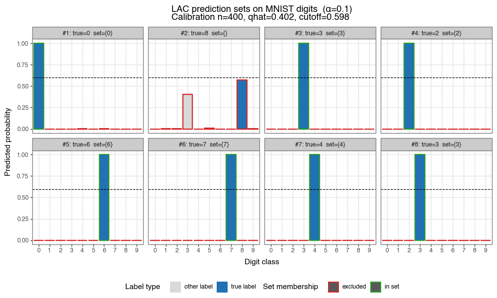
Each panel shows predicted probabilities for a test image. Blue = true label, green = other classes in prediction set, grey = excluded. The dashed black line marks the LAC inclusion cutoff \(1-\hat{q}\): classes above this line are included in the prediction set.
(2.3a) Comparative view: LAC vs APS in score space
The figure below shows four different test images, each with three columns comparing LAC, randomized APS (U ~ Uniform(0,1)), and deterministic APS (U=0). This visualization makes the different scoring logic transparent.
LAC column (left):
- Bars show the model’s predicted probabilities in the original class order (0–9).
- Dashed line is the inclusion cutoff $1-\hat{q}$: classes above this line (green borders) are in the prediction set.
- The decision rule is simple: use a global threshold.
APS columns (middle and right):
- Classes are sorted by descending probability: the highest-probability class is labeled 0, the next is 1, etc.
- Bars still show individual class probabilities (the height of each bar is the original model’s softmax).
- Purple line: cumulative probability $\sum_{j \le k} p_{(\pi_j)}$, where $(\pi_1), (\pi_2), \ldots$ is the sorted order.
- Orange dots: the realized APS nonconformity score for each class, $s_{APS}(x, c) = \text{cumsum}_c - U_c \cdot p_c$.
- For deterministic APS, $U_c = 0$, so the orange dots exactly follow the purple line.
- For randomized APS, $U_c$ is drawn once per test image; you see the unique realization as a label (
u_true=...) in the first bar.
- Dashed line: $\hat{q}$, the conformal threshold. Classes whose APS score (orange dot) falls below the dashed line are included in the prediction set.
Key insight: The APS score “consumes” probability mass as you move down the ranked list. A class near the top of the ranking (say, position 2) has a lower cumulative sum and is thus less likely to exceed $\hat{q}$. A class near the bottom (position 9) has burned through all prior probability and is unlikely to be included. This ranking-based logic makes APS adaptive: it naturally biases toward high-probability classes while automatically expanding the set when the model is uncertain (flat probabilities, high cumsum).
Figure 1b: LAC vs APS variants in score space (α=0.10)
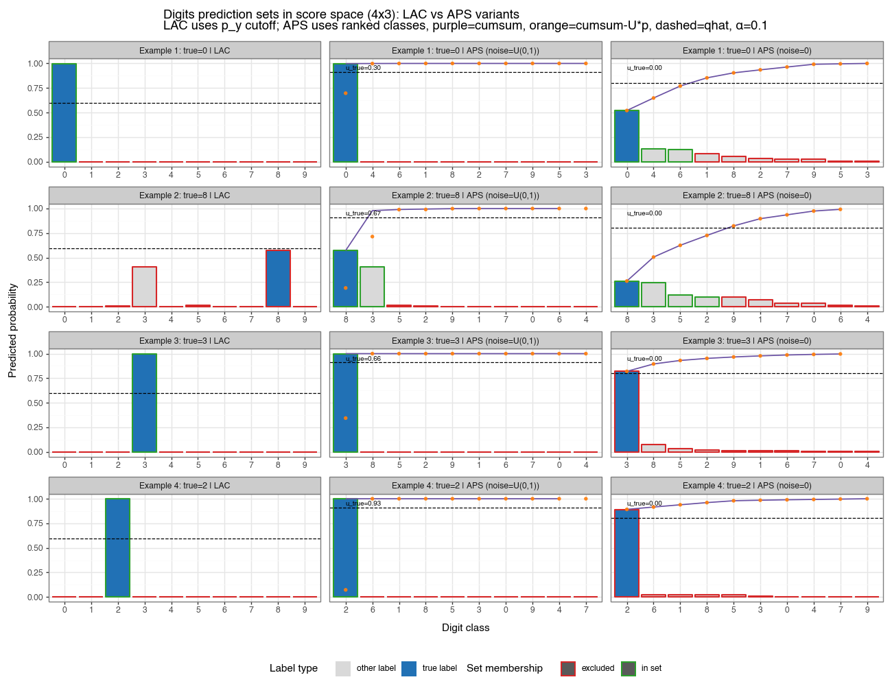
4×3 grid: rows = four test examples, columns = LAC / APS randomized / APS deterministic. LAC uses a global probability cutoff (dashed line at 1−q̂). APS ranks classes by probability and plots cumulative probability (purple line) and realized NCS scores (orange dots); inclusion is determined by score ≤ q̂. For randomized APS, the label u_true shows the uniform random draw for that example. The color coding (green = in set, grey = excluded, blue = true label) is consistent across all three methods.
(2.4) Simulation: LAC vs APS — same coverage, different efficiency
The following simulation compares LAC, deterministic APS (noise=0), and the textbook randomized APS (noise=U(0,1)) across 500 independent trials on a synthetic \(k=6\) class multinomial problem. In each trial, a logistic regression is trained on \(n_{\text{train}}=250\) observations, calibrated on \(n_{\text{cal}}=500\), and evaluated on \(n_{\text{val}}=100\) test points.
from utils import dgp_multinomial, NoisyGLM, simulation_cp

p, k, alpha = 5, 6, 0.10
dgp = dgp_multinomial(p, k, snr=0.6*k, seeder=42)

for score_name, score_cls, score_kwargs in [
    ('LAC', score_lac, {}),
    ('APS (noise=0)', score_aps, {'noise': 0.0, 'random_state': 42}),
    ('APS (noise=U(0,1))', score_aps, {'noise': 'uniform', 'random_state': 42}),
]:
    mdl = NoisyGLM(max_iter=250, noise_std=0.0, seeder=42,
                   subestimator=LogisticRegression, penalty=None)
    cp  = conformal_sets(f_theta=mdl, score_fun=score_cls, alpha=alpha, **score_kwargs)
    sim = simulation_cp(dgp=dgp, ml_mdl=mdl, cp_mdl=cp, is_classification=True)
    res = sim.run_simulation(n_train=250, n_calib=500, n_test=100, nsim=500, seeder=42)
    print(f'{score_name}: cover={100*res.cover.mean():.1f}%  set_size={res.set_size.mean():.2f}')
# LAC: cover=90.1%  set_size=1.18
# APS (noise=0): cover=90.2%  set_size=2.65
# APS (noise=U(0,1)): cover=90.3%  set_size=1.34
The figure below shows two things: (a) the empirical coverage histogram against the theoretical beta-binomial distribution, and (b) the distribution of average set sizes. All three methods shown here — LAC, deterministic APS, and randomized APS — achieve the nominal 90% marginal coverage and match the beta-binomial prediction closely. The additional comparison above isolates the effect of APS randomization itself: here the deterministic version (noise=0) is slightly more conservative and materially less efficient, with average set size 2.65 versus 1.34 for the textbook randomized version. The broader efficiency comparison with LAC still depends on the problem. When the model is well-calibrated and classes are well-separated, LAC’s sharp thresholding is efficient. When the model is uncertain, APS produces sets that better reflect the local uncertainty structure by adding classes in order of decreasing probability.
Figure 2a: Empirical coverage vs beta-binomial theory
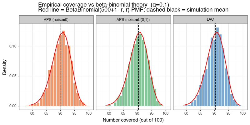
Histogram of empirical coverage counts (out of 100 test points) across 500 simulations for LAC, deterministic APS, and randomized APS. The red line shows the theoretical beta-binomial PMF, and all three methods track it closely.
Figure 2b: Prediction set size — LAC vs APS variants
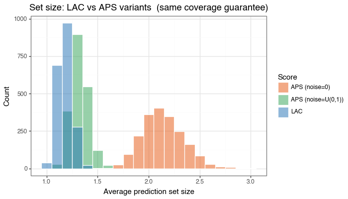
Overlaid histogram of average prediction set sizes with semi-transparent bars. All three methods satisfy the same coverage constraint; deterministic APS is the least efficient here, while randomized APS removes much of that excess conservatism.
(2.5) Coverage as a function of \(\alpha\)
The marginal coverage guarantee is \(P(Y \in \mathcal{C}(X)) \geq 1 - \alpha\) for any \(\alpha\). The figure below sweeps \(\alpha\) from 0.05 to 0.30 and shows the empirical coverage achieved (LAC, same synthetic problem). The empirical mean tracks the nominal level \(1-\alpha\) (dashed line) throughout, with the 10th–90th percentile ribbon tightening as \(\alpha\) increases and uncertainty about \(\hat{q}\) is lower.
Figure 3: Empirical coverage vs nominal level (LAC)
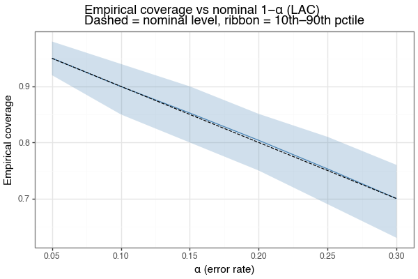
Mean empirical coverage (solid) tracks the nominal 1−α (dashed) at all error rates. Ribbon shows 10th–90th simulation percentile. n_calib=500 in all cases.
(3) Regression: three non-conformity scores
For a continuous outcome \(Y \in \mathbb{R}\), the conformal prediction set is an interval \([L(x), U(x)]\). Three methods are described below, in order of increasing adaptivity to heteroskedasticity.
(3.1) Simple residual score (MAE)
The most natural NCS for regression is the absolute residual:
\[s_{\text{MAE}}(x, y) = |y - \hat{f}(x)|\]The calibration step finds \(\hat{q}\) from the calibration residuals, and prediction intervals are symmetric around \(\hat{f}\):
\[\mathcal{C}_{\text{MAE}}(x) = \left[ \hat{f}(x) - \hat{q},\; \hat{f}(x) + \hat{q} \right]\]The interval width is constant across all \(x\): every test point receives the same \(\pm \hat{q}\) band. This is efficient when the noise variance is homoskedastic (constant across \(x\)), but wasteful when variance depends on \(x\): low-noise regions get unnecessarily wide intervals, and high-noise regions may be too tight.[3]
(3.2) Studentized score (locally-weighted residuals)
To adapt interval widths to local uncertainty, fit a second model \(\hat{\sigma}(x)\) that predicts the expected scale of residuals. The studentized NCS (LGRTW18) is:
\[s_{\text{stud}}(x, y) = \frac{|y - \hat{f}(x)|}{\hat{\sigma}(x)}\]With a single calibration quantile \(\hat{q}\), the prediction interval becomes:
\[\mathcal{C}_{\text{stud}}(x) = \left[ \hat{f}(x) - \hat{q}\cdot\hat{\sigma}(x),\; \hat{f}(x) + \hat{q}\cdot\hat{\sigma}(x) \right]\]Now interval width scales with \(\hat{\sigma}(x)\): regions where the model is locally uncertain get wider intervals, and confident regions get narrower ones. The marginal coverage guarantee still holds exactly as before — the studentized score is just a different NCS, and the conformal calibration is agnostic to the form of the score.
In practice, there are at least three common ways to obtain \(\hat{\sigma}(x)\):
- Native model support. Some models directly output both a mean and uncertainty/scale estimate (for example, Gaussian Process Regression or a neural network trained with a Gaussian likelihood that predicts mean and log-variance jointly).
- Implied model variance. Some pipelines derive uncertainty from model randomness or posterior structure (for example, MC-dropout dispersion, ensemble variance, or Bayesian posterior predictive variance).
- Auxiliary scale model. Fit a second model to first-stage errors, usually \(|y_i - \hat{f}(x_i)|\), so the first model learns location and the second learns local scale (stacking-style).
This post uses the third option because it is simple, model-agnostic, and works with any base regressor that has a predict method. A ridge or gradient boosting regressor is a reasonable second-stage choice for the auxiliary scale model.
In practice, the second-stage target is often one of three transforms of first-stage errors: \(|e_i|\), \(e_i^2\), or \(\log(e_i^2+\varepsilon)\), where \(e_i = y_i-\hat{f}(x_i)\). These are all monotone surrogates of local noise scale and therefore carry similar information about where uncertainty is high or low. Importantly, studentized conformal is scale-equivariant: if \(\hat{\sigma}(x)\) is off by a constant factor \(c>0\), then scores \(|e|/\hat{\sigma}(x)\) are rescaled by \(1/c\), and the calibrated quantile \(\hat{q}\) rescales by the same factor. The final interval width \(\hat{q}\cdot\hat{\sigma}(x)\) is therefore unchanged up to this global constant, so getting the relative shape of \(\hat{\sigma}(x)\) over \(x\) is usually more important than perfect absolute calibration.
from sklearn.linear_model import LinearRegression, Ridge
from conformal import conformal_sets, score_studentized
from utils import StudentizedEstimator

mean_mdl  = LinearRegression()
scale_mdl = Ridge(alpha=1.0)
stud_est  = StudentizedEstimator(mean_mdl, scale_mdl)
stud_est.fit(X_train, y_train)

cp = conformal_sets(f_theta=stud_est, score_fun=score_studentized, alpha=0.10)
cp.fit(x=X_cal, y=y_cal)
intervals = cp.predict(X_test)  # shape (n_test, 2): columns are [lower, upper]
(3.3) Conformalized Quantile Regression (CQR)
A third approach trains quantile regression models \(\hat{q}_{\alpha/2}(x)\) and \(\hat{q}_{1-\alpha/2}(x)\) directly, then uses the pinball score (RPC19):
\[s_{\text{CQR}}(x, y) = \max\!\left(\hat{q}_{\alpha/2}(x) - y,\;\; y - \hat{q}_{1-\alpha/2}(x)\right)\]This score is positive when \(y\) falls outside the uncalibrated quantile interval, and negative when inside. The conformal calibration finds \(\hat{q}\) from the calibration scores, and the final interval is:
\[\mathcal{C}_{\text{CQR}}(x) = \left[ \hat{q}_{\alpha/2}(x) - \hat{q},\;\; \hat{q}_{1-\alpha/2}(x) + \hat{q} \right]\]When the quantile regression model is well-specified, the uncalibrated interval already has approximately \(1-\alpha\) coverage and \(\hat{q} \approx 0\). The conformal step provides the marginal coverage guarantee as a correction, while the quantile model provides the adaptivity. CQR has the appealing property that the intervals are asymmetric: \(y - \hat{q}_{1-\alpha/2}\) and \(\hat{q}_{\alpha/2} - y\) can have different magnitudes depending on the conditional distribution of \(Y \vert X\).
from utils import QuantileRegressors, LinearQuantileRegressor
from conformal import conformal_sets, score_pinpall

alpha = 0.10
mdl = QuantileRegressors(subestimator=LinearQuantileRegressor,
                         alphas=[alpha/2, 1 - alpha/2])
mdl.fit(X_train, y_train)

cp = conformal_sets(f_theta=mdl, score_fun=score_pinpall, alpha=alpha)
cp.fit(x=X_cal, y=y_cal)
intervals = cp.predict(X_test)
(3.4) Simulation: marginal vs conditional coverage
A simulation using a heteroskedastic data generating process illustrates the key difference between the three methods. The DGP is:
\[Y_i = X_i^\top \beta + \varepsilon_i, \quad \varepsilon_i \sim \mathcal{N}\!\left(0,\; \exp(X_i^\top \gamma / p)^2 \cdot \sigma_0^2 \right)\]where \(\gamma\) is a fixed random vector, so the noise variance varies exponentially across the input space. We split the test observations into low-noise and high-noise terciles based on their true \(\sigma(x)\), and measure conditional coverage and interval width separately in each group.
All three methods maintain the nominal 90% marginal coverage. The difference is in conditional coverage. The simple MAE score, by construction, uses a single constant radius \(\hat{q}\): it achieves ~95% coverage in the low-noise tercile (overly conservative, wasteful) and only ~84% in the high-noise tercile (under-covers where it matters most). The studentized and CQR scores adapt their widths to the local noise level, achieving approximately 90% coverage in both terciles.
Figure 4a: Conditional coverage by noise level across 200 simulations
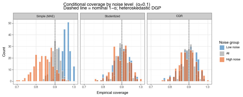
Histogram of empirical coverage rates, broken out by noise tercile (blue=low, orange=high). All methods achieve ~90% marginal coverage (grey). Simple MAE systematically over-covers low-noise regions and under-covers high-noise regions. Studentized and CQR are calibrated in both.
Figure 4b: Interval widths by noise level
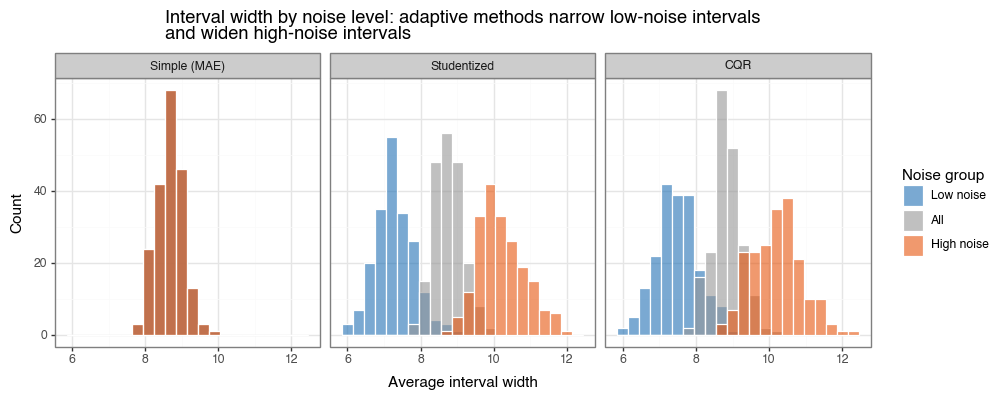
Interval widths for low-noise (blue) and high-noise (orange) subgroups. Simple MAE produces identical widths in both groups. Studentized and CQR narrow intervals in low-noise regions and widen them in high-noise regions — the hallmark of efficient heteroskedastic coverage.
(3.5) Real data example: Diabetes dataset
The Diabetes dataset (Efron et al. 2004) has \(n=442\) observations and 10 quantitative predictors. It exhibits mild heteroskedasticity. The plot below shows prediction intervals for the three methods on \(n_{\text{test}} = 92\) held-out observations, sorted by their true response value. The black ✕ marks show true response values; intervals are colored by method.
Figure 5: Prediction intervals on the Diabetes dataset (α=0.10)
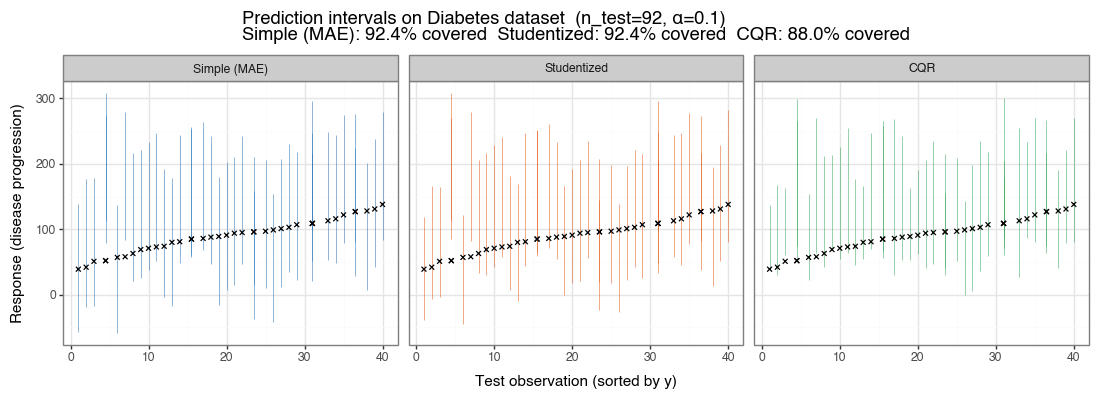
n_train=250, n_calib=100. First 40 test observations (sorted by true response) shown for clarity. CQR intervals are visibly asymmetric and narrower in the lower response range where variance is lower.
(3.6) Conformalizing Bayes: density NCS and HDR sets
When a model natively defines a conditional density \(f(y \mid x;\theta)\), conformalization can be done directly in density space using
\[s_{\text{dens}}(x,y) = -\log f(y \mid x;\theta).\]After calibration, let \(\hat{q}\) be the conformal quantile of these scores and define \(\log\tau = -\hat{q}\). The conformal prediction set is then the density superlevel set
\[\mathcal{C}(x) = \{y: \log f(y\mid x;\theta) \ge \log\tau\},\]which is exactly a highest-density-region (HDR)-style construction under a data-driven threshold chosen to enforce finite-sample marginal coverage.
The geometric shape of this set depends on posterior shape:
| Posterior shape | Prediction set |
|---|---|
| Unimodal symmetric (e.g. Gaussian) | Single interval \([a, b]\) |
| Unimodal asymmetric (e.g. log-normal) | Single interval \([a, b]\), often touching a support boundary |
| Monotone decreasing (e.g. Exponential) | \([0, b]\) with left endpoint at support boundary |
| \(k\)-modal | Union of \(k\) disjoint intervals \([a_1,b_1] \cup \cdots \cup [a_k,b_k]\) |
| Threshold above density peak | Empty set (degenerate; rare under well-calibrated in-distribution use) |
For this first implementation, I use a unimodal interval solver: evaluate \(g(y)=\log f(y\mid x)-\log\tau\) on a grid, bracket sign changes, refine roots with Brent’s method, and return the interval hull of the superlevel region.
On California Housing, this approach achieved empirical coverage 0.904 on a held-out test split at \(\alpha=0.10\) (so target 0.90), with mean interval width 1.342 and empty-set rate 0.0%. Across 250 repeated train/calibration/test resamples, mean coverage was 90.2%, consistent with conformal validity.
Figure 6a: Conformalizing Bayes coverage vs beta-binomial reference
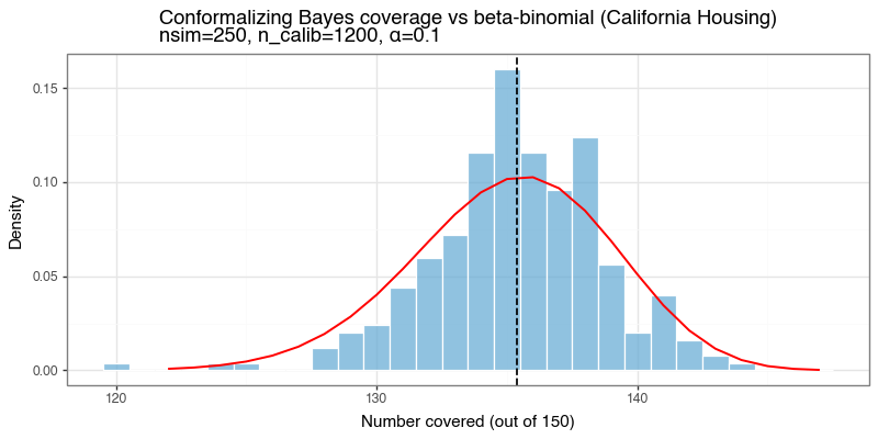
Coverage-count histogram across repeated resamples for density-based conformal intervals on California Housing. The red line is the beta-binomial reference induced by calibration quantile randomness.
Figure 6b: Distribution of HDR interval widths
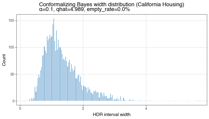
Width distribution for test-set HDR intervals from the conformalized density model (single split). Width variability reflects local uncertainty captured by \(f(y\mid x;\theta)\).
Figure 6c: Root-solved HDR examples on individual instances
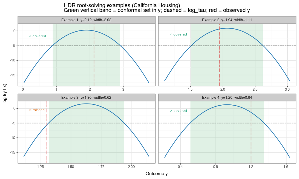
Each panel shows \( \log f(y\mid x) \) vs. \(y\) for one test instance. The dashed horizontal line is \(\log\tau\). The green vertical band marks the conformal prediction set in \(y\) (the superlevel set projected to the x-axis), and the red vertical line is the observed response. The in-panel annotation uses ✓ for covered and \(\times\) for missed.
(3.7) Localized conformal prediction (baseLCP + LOO PIT)
The adaptive methods described so far — studentized and CQR — keep the conformal quantile \(\hat{q}\) global (a single number calibrated once on the whole calibration set) and instead adapt the interval by learning an auxiliary model for local scale or quantiles. An alternative strategy is to adapt the quantile itself: rather than asking “what is the \((1-\alpha)\)-quantile of all calibration scores?”, ask “what is the \((1-\alpha)\)-quantile of scores near \(x\)?”. Localized conformal prediction pursues this idea by computing a covariate-specific threshold \(\hat{q}(x)\) that varies continuously across the input space.
The baseLCP idea
The core idea (Guan, 2023) is to replace the flat empirical quantile with a Nadaraya–Watson (NW) kernel-weighted quantile. A kernel \(H(x_i, x)\) is a measure of similarity between two points: it returns a large value when \(x_i\) is close to \(x\) and a small value when they are far apart. Normalizing these similarities gives a probability weight for each calibration point:
\[w_i(x) = \frac{H(X_i, x)}{\sum_{j=1}^{n} H(X_j, x)},\]and the local threshold is the weighted \((1-\alpha)\)-quantile of the calibration scores under those weights:
\[\hat{q}_{1-\alpha}(x) = \text{Quantile}_{1-\alpha}\!\left(\sum_{i=1}^{n} w_i(x)\,\delta_{V_i}\right).\]This is a weighted empirical quantile: calibration points near \(x\) dominate, distant ones are down-weighted, so the threshold adapts to the local distribution of scores. The standard choice is the Gaussian RBF kernel \(H(x_i, x) = \exp(-|x_i - x|^2 / 2h^2)\), which assigns similarity that decays smoothly with squared Euclidean distance; the bandwidth \(h\) controls how quickly that decay happens. We use this kernel throughout.
LOO PIT: debiased calibration scores
Directly applying a kernel-weighted quantile of \(V_i\) at test points works, but produces calibration scores that are not well-calibrated to \(\text{Unif}(0,1)\) because the kernel CDF evaluated at its own training points is biased upward (an in-sample effect analogous to training-set R²). To reduce this bias we transform calibration scores to probability integral transform (PIT) values using leave-one-out (LOO) kernel CDFs.
The entire calibration split \({(X_i, V_i)}_{i=1}^n\) is used for two steps:
Step A — bandwidth selection. We grid-search over \(h\) and choose
\[h^* = \arg\min_h \sum_{i=1}^n \bigl(V_i - \hat{m}_{-i,h}(X_i)\bigr)^2,\]where \(\hat{m}_{-i,h}(x)\) is the LOO NW regression estimate of \(V\) at \(x\), computed from all calibration points except \(i\). This is the standard LOO cross-validation criterion for NW regression, and it selects the bandwidth that best predicts NCS in new-to-the-neighborhood points.
Step B — LOO PIT scores. With \(h^*\) fixed, compute
\[\tilde{V}_i = \hat{F}_{-i}(V_i \mid X_i;\, h^*) \;=\; \sum_{j \neq i} w_j^{(-i)}(X_i)\,\mathbf{1}(V_j \leq V_i),\]where \(w_j^{(-i)}\) are kernel weights from \(X_i\) to all other calibration points. Standard split-conformal calibration is then run on \(\tilde{V}_1,\ldots,\tilde{V}_n\) to obtain \(\hat{q}\).
Bias caveat. Using the same calibration set for both bandwidth selection (Step A) and PIT scoring (Step B) leaves a mild bias: \(h^*\) is fit to the same points whose LOO PIT scores we then evaluate. The LOO construction removes the most egregious within-sample optimism, but does not eliminate it entirely. A fully unbiased procedure would estimate \(h\) on a separate training fold; here we accept the residual bias as a practical tradeoff and call it out explicitly.
Test-time inversion
At a new test point \(x_{\text{new}}\), the full calibration set (no LOO needed) is used to estimate the kernel CDF:
\[\hat{F}(v \mid x_{\text{new}};\,h^*) = \sum_{i=1}^{n} w_i(x_{\text{new}})\,\mathbf{1}(V_i \leq v).\]The local threshold is \(\tau(x_{\text{new}}) = \hat{F}^{-1}(\hat{q} \mid x_{\text{new}})\), inverted by finding the smallest calibration NCS value whose cumulative kernel weight reaches \(\hat{q}\). The final interval is
\[\mathcal{C}(x_{\text{new}}) = \bigl[\hat{\mu}(x_{\text{new}}) - \tau(x_{\text{new}}),\;\hat{\mu}(x_{\text{new}}) + \tau(x_{\text{new}})\bigr],\]where \(\hat{\mu}\) is the mean model’s prediction.
What baseLCP does not guarantee — and how variants fix it
baseLCP does not guarantee marginal coverage in general. The PIT-calibrated quantile \(\hat{q}\) is chosen on transformed scores and produces a test-time threshold that adapts locally, but the exchangeability argument that underlies conformal validity does not apply when the threshold itself is a function of \(x\).
The main methods that address this small but real gap are:
| Variant | Core fix | Key tradeoff |
|---|---|---|
| calLCP (Guan 2023) | Recalibrates the effective level \(\tilde\alpha\) so the marginal empirical coverage over calibration points hits \(1-\alpha\) exactly | May over-cover in low-noise regions to compensate for under-coverage elsewhere |
| RLCP (Hore & Barber 2025) | Centers kernel weights at a randomized prototype \(\tilde{X}_{n+1}\sim p_H(\cdot\mid X_{n+1})\) rather than at the true test point; restores exchangeability | Intervals are averages over the random prototype draw, so local adaptation is slightly smoothed |
| DCP / HPD-split (Chernozhukov et al. 2021; Izbicki et al. 2022) | Transform scores via \(\tilde V_i=\hat F_Y(Y_i\mid X_i)\) (the full conditional CDF of \(Y\)); asymptotically \(\tilde V\sim\text{Unif}(0,1)\) for all \(X\) simultaneously, making a single global threshold work locally | Requires estimating \(\hat F_Y(\cdot\mid x)\), e.g. via quantile regression; gains are asymptotic, not finite-sample |
Results on California Housing
On the same California Housing split used for the Bayes section (same train/calibration/test partition and scaler), the localized method uses the concatenated feature vector \((X, \hat{\mu}(X))\) as the kernel input (normalized before computing distances). It selected \(h^*=0.714\), achieved empirical coverage 0.902 at \(\alpha=0.10\), and produced mean interval width 1.504 — narrower than the Bayes HDR method (1.519). Across 200 repeated resamples, the coverage distribution follows the beta-binomial reference closely.
The table below breaks down coverage and mean width by decile of the true response, comparing the Bayes HDR (Section 3.6) and localized methods on the same test set.
| Decile | y range | n | Bayes cov | Bayes width | Local cov | Local width |
|---|---|---|---|---|---|---|
| D1 | [0.15, 0.82) | 1611 | 0.932 | 1.138 | 0.918 | 1.078 |
| D2 | [0.82, 1.07) | 1616 | 0.951 | 1.221 | 0.934 | 1.140 |
| D3 | [1.07, 1.34) | 1612 | 0.952 | 1.289 | 0.937 | 1.208 |
| D4 | [1.34, 1.57) | 1611 | 0.944 | 1.341 | 0.926 | 1.259 |
| D5 | [1.57, 1.80) | 1615 | 0.950 | 1.411 | 0.946 | 1.346 |
| D6 | [1.80, 2.09) | 1615 | 0.940 | 1.529 | 0.933 | 1.502 |
| D7 | [2.09, 2.42) | 1616 | 0.939 | 1.646 | 0.935 | 1.671 |
| D8 | [2.42, 2.91) | 1615 | 0.915 | 1.759 | 0.903 | 1.843 |
| D9 | [2.91, 3.80) | 1615 | 0.848 | 1.899 | 0.854 | 2.035 |
| D10 | [3.80, 5.00] | 1614 | 0.709 | 1.952 | 0.731 | 1.952 |
| Overall | 16140 | 0.908 | 1.519 | 0.902 | 1.504 |
Both methods struggle at the high end of the response (D10: \(y > 3.8\)), reflecting genuinely harder cases. The localized method achieves narrower widths in D1–D5 (low-response region) and is modestly wider in D7–D9, with comparable overall coverage. The 1% reduction in mean width relative to Bayes comes from the kernel adapting to residual structure in \((X, \hat{\mu})\)-space.
Figure 7a: Localized conformal interval widths
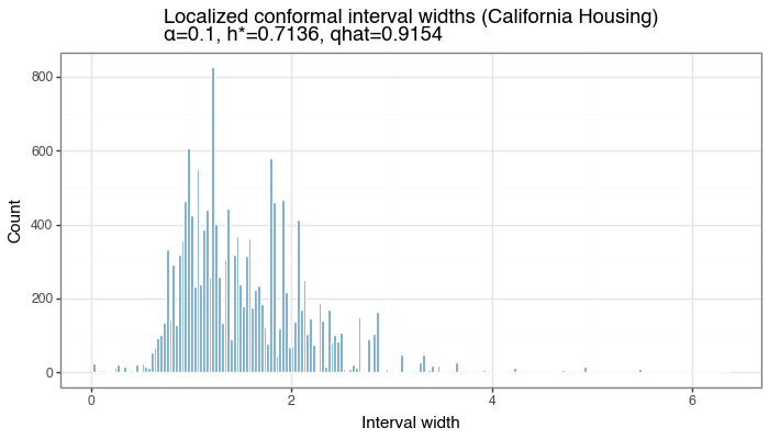
Distribution of per-test-point interval widths from baseLCP + LOO PIT on California Housing (single split). Width variability reflects how much \(\tau(x)\) adapts to local density of calibration scores.
Figure 7b: Example localized prediction intervals
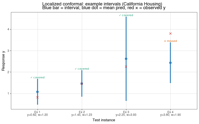
Four test instances at the 10th, 35th, 65th, and 90th percentile of the true response. Blue bar = localized interval; red ✕ = observed \(y\). In-panel annotation uses ✓ for covered and \(\times\) for missed.
Figure 7c: Width correlation — Bayes vs Localized
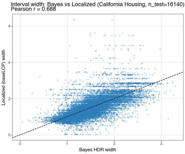
Scatter of per-test-point interval widths from conformalizing Bayes (x-axis) vs baseLCP + LOO PIT (y-axis) on the same test set. Points near the 1:1 line (dashed) indicate the two methods agree on which inputs are uncertain; deviations reflect different uncertainty decompositions (density-model vs kernel-quantile).
Figure 7d: Coverage distribution vs beta-binomial reference
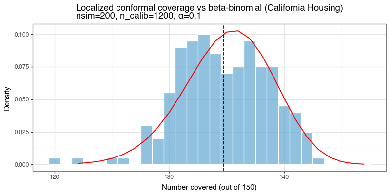
Coverage-count histogram across 200 repeated resamples. The red line is the beta-binomial reference. baseLCP + LOO PIT tracks the reference well despite the lack of a formal marginal-coverage guarantee.
(4) Limitations
(4.1) Exchangeability is the load-bearing assumption
The coverage guarantee rests on a single probabilistic assumption: that the calibration and test data are exchangeable. Everything else — the choice of model, the non-conformity score, the data distribution — is unconstrained. The framework’s breadth therefore lives or dies with this one condition, and in practice it is the condition most likely to fail.
Exchangeability is roughly the requirement that no ordering structure distinguishes calibration points from test points: if you shuffled all of them together, no statistical test could tell which were which. This holds automatically when both sets are i.i.d. draws from the same distribution, but fails in many common deployment patterns. Consider temporal drift: a model calibrated on data from one quarter of the year may face a shifted input distribution several months later due to seasonality, policy changes, or population evolution. The calibration scores were computed under one regime; the test scores arise under another. The quantile threshold \(\hat{q}\) is miscalibrated for the new regime, and the nominal \(1-\alpha\) guarantee no longer holds — coverage can be substantially below target without any warning from the procedure itself. The same logic applies to covariate shift more broadly, where \(P(X)\) changes between calibration and deployment while \(P(Y \mid X)\) may or may not remain stable. It also applies to batch effects in scientific data: if calibration samples were processed in one laboratory or on one instrument run and test samples arrive from a different batch, systematic technical variation can create a distributional gap even when the underlying signal is identical. Transfer learning settings introduce a related problem: a model pre-trained on a source domain and calibrated on a small target-domain set may have well-calibrated coverage within the target domain, but if the target domain itself is heterogeneous the exchangeability assumption may still be only approximate.
(4.2) Violations are often silent and can hide subgroup failures
An important subtlety is that violations of exchangeability are often silent. The conformal procedure will produce a prediction set for every test input regardless; it does not flag that its own guarantee has lapsed. A practitioner who does not actively monitor marginal coverage on recent holdout data could be operating outside the guarantee without realising it. Worse, because the guarantee is marginal, even correct average coverage can conceal systematic under-coverage in the subpopulations that matter most — a model deployed in a hospital might achieve 90% coverage on the overall test population while covering only 80% for the sickest patients, if those patients are systematically underrepresented in the calibration data.
(4.3) Coverage is a property of the procedure, not a given interval
Two further gotchas are worth stating explicitly, because they are frequently misunderstood in practice.
The first concerns what “coverage” actually means. The guarantee \(P(Y_{n+1} \in \mathcal{C}(X_{n+1})) \geq 1 - \alpha\) is a statement about the procedure, not about any individual prediction set. More precisely, it is a statement about the next exchangeable draw: if you re-ran the entire process — drawing a fresh calibration set, recomputing \(\hat{q}\), and predicting on a new test point — the resulting set would contain the true label at least \(1-\alpha\) fraction of the time in expectation over that randomness. Once \(\hat{q}\) has been fixed and a specific \(\mathcal{C}(x)\) has been produced, that interval either covers the true value or it does not. There is no probability left; the uncertainty has collapsed. This is directly analogous to the classical confidence interval misconception: a 95% confidence interval does not mean there is a 95% probability that the true parameter lies inside this particular interval — it means that the interval-construction procedure would capture the true value in 95% of repeated applications. A conformal prediction set carries exactly the same caveat. Researchers who interpret \(\mathcal{C}(x)\) as having a \(1-\alpha\) posterior probability of covering \(Y\) are importing a Bayesian interpretation into a frequentist guarantee that does not support it.
This is also why larger calibration sets are so valuable in practice, even for the simplest \(\pm\hat{q}\) interval. The deployment-level coverage for a fixed fitted model, \(\theta(\mathcal{D}_{\text{cal}})=P(Y\in\mathcal{C}(X)\mid\mathcal{D}_{\text{cal}})\), is random because \(\hat{q}\) is random. Across repeated calibrations, some deployed models will over-cover and some will under-cover relative to 90% (with a slight conservative tilt from finite-sample quantile adjustment). Increasing \(n_{\text{calib}}\) concentrates this distribution of \(\theta(\mathcal{D}_{\text{cal}})\) around \(1-\alpha\), so typical realized coverage gets closer to target: e.g., the kind of miss that might be 86% with a very small calibration set can move much closer to 89–90% when calibration is larger.
The second concerns batches of predictions. Suppose you deploy the model and observe \(m\) new test points simultaneously. Each individual coverage event \(\mathbf{1}[Y_i \in \mathcal{C}(X_i)]\) has marginal probability at least \(1-\alpha\), but the joint distribution of the \(m\) coverage indicators is not specified by the conformal guarantee alone. In the simplest case — where the \(m\) test points are exchangeable with each other and with the calibration set, and the same \(\hat{q}\) is applied to all — the total number of covered test points follows approximately \(\text{Binomial}(m, 1-\alpha)\) in expectation. That has mean \(m(1-\alpha)\) and standard deviation \(\sqrt{m \alpha (1-\alpha)}\), so for any particular batch of \(m\) predictions the realised coverage rate will deviate from \(1-\alpha\) by \(O(1/\sqrt{m})\). For \(m = 100\) and \(\alpha = 0.1\) the standard deviation of the number covered is \(\sqrt{100 \times 0.1 \times 0.9} \approx 3\), meaning the realised coverage rate for that batch routinely fluctuates between roughly 87% and 93%. This is not a failure of conformal prediction — it is binomial sampling noise — but it means that evaluating a deployed system on a single batch of moderate size and concluding it “achieves 90% coverage” or “misses the target” requires care. The beta-binomial distribution described in Section 1.4 makes this sampling variability precise and provides a rigorous diagnostic for whether observed deviations are consistent with the nominal guarantee.
(4.4) Methods that relax exchangeability
There is a large and active literature working to relax or adapt the exchangeability requirement. Weighted conformal prediction (Tibshirani et al., 2019) re-weights calibration scores by an estimated likelihood ratio between the calibration and test distributions, recovering approximate coverage under covariate shift when the density ratio can be estimated. Mondrian conformal prediction stratifies calibration by a grouping variable and constructs separate thresholds per stratum, trading off global calibration size for within-group coverage. Online and adaptive conformal prediction methods (Gibbs & Candès, 2021) update \(\hat{q}\) sequentially as new observations arrive, allowing the coverage level to track a drifting distribution over time. Calibration under label shift, conformal risk control, and various robust variants address yet other departures from the basic setup. A detailed treatment of these methods and the conditions under which they provide guarantees is left for a future post; the take-away here is that exchangeability should always be treated as an assumption to be actively scrutinised rather than a background fact about the data.
(5) Discussion
What conformal prediction gives you. The marginal coverage guarantee holds with no assumptions on the data distribution, the model class, or the model’s calibration. It is valid for neural networks, gradient boosting, or any other black-box predictor (including a random number generator). The guarantee is finite-sample and non-asymptotic — 90% means 90% with \(n = 100\) calibration points, not just in the limit (although again this is in expectation).
What it does not give you. Marginal coverage is an average over test inputs. If the prediction set is very wide in some regions and narrow in others, it can still satisfy the marginal guarantee while being practically useless for individual predictions. The studentized and CQR methods move closer to conditional coverage by adapting intervals to local uncertainty, but neither achieves exact conditional coverage. This is not a limitation of the specific methods chosen — it is a fundamental impossibility result[4]: no distribution-free method can guarantee \(P(Y \in \mathcal{C}(X) \mid X = x) \geq 1 - \alpha\) for all \(x\) without placing assumptions on the underlying distribution (BCRT21). Intuitively, estimating coverage at a specific \(x\) requires enough calibration points in the neighbourhood of \(x\), which for a continuous covariate space is never finite.
Epistemic vs aleatoric uncertainty. The width of a conformal prediction interval reflects total predictive uncertainty and cannot be decomposed into epistemic uncertainty (arising from limited data or a mis-specified model) and aleatoric uncertainty (irreducible noise in \(Y \mid X\)). A wide interval might mean the model is poorly identified, the training set is too small, or simply that \(Y \mid X\) is inherently noisy — conformal prediction cannot distinguish these. Separating the two components requires stronger scaffolding: explicit distributional assumptions about the DGP, an auxiliary source of variance information (e.g. replicate measurements of the same \(x\), which directly reveal \(\text{Var}(Y \mid X = x)\)), or a full probabilistic model whose posterior can be used to estimate parameter uncertainty separately. None of this is available within the distribution-free conformal framework, which is precisely what makes the coverage guarantee so broadly applicable.
Average prediction set size is mostly driven by the base model; conformal mostly controls adaptivity. If prediction intervals are too wide to be actionable, the dominant driver is usually base-model error scale (or weak signal in the features), and conformal calibration is reporting that uncertainty under a valid coverage constraint. A conformal predictor that outputs \({3, 5, 7}\) for an ambiguous digit, or a regression interval spanning half the response range, is often an honest signal that the underlying predictor cannot localize outcomes well for those inputs. Better features, better model class, or more data typically move the average set size the most. Different conformal scores/methods can still produce meaningful efficiency gains — as we showed in this post — but these gains are often more about where width is allocated (better local adaptivity) than large changes in overall average width.
-
Every i.i.d. sequence is exchangeable, but not every exchangeable sequence is i.i.d. A canonical counterexample is a finite population sample without replacement: if \((X_1, \ldots, X_n)\) are drawn without replacement from a fixed urn, any permutation of the draws has the same joint distribution, so the sequence is exchangeable — but the draws are not independent (knowing \(X_1\) changes the distribution of \(X_2\)). Conformal prediction only requires the calibration and test points to be exchangeable with one another, which holds whenever they are an i.i.d. sample but also in the without-replacement setting and other non-i.i.d. scenarios. ↩
-
In practice, the calibration set may be the only set a researcher needs. For example, the fitted model may be model weights downloaded from an external source, and there’s no requirement per se to test if the coverage guarantees hold on an evaluation set. ↩
-
A mean squared error (MSE) score \(s_{\text{MSE}}(x,y) = (y - \hat{f}(x))^2\) is equivalent up to a monotone transformation: \(\hat{q}_{\text{MSE}}^{1/2} = \hat{q}_{\text{MAE}}\), so the two produce identical intervals. MAE is more common in the literature. ↩
-
The impossibility of exact distribution-free conditional coverage was formally established by Foygel Barber, Candès, Ramdas & Tibshirani, “The limits of distribution-free conditional predictive inference”, Bernoulli 2021. In their Section 2.2 they credit two prior sources for the underlying observation: Vovk (2012), “Conditional validity of inductive conformal predictors” (ACML 2012), who first raised the issue in the conformal prediction setting; and Lei & Wasserman (2014), “Distribution-free prediction bands for non-parametric regression” (JRSS-B), who discuss the marginal/conditional gap in the context of nonparametric regression bands. ↩